Numeric integration¶

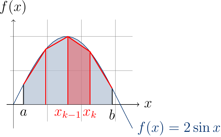
In numeric integration, one aims to compute (an approximate) solution of a definite integral. One of the simplest method is to use the trapezoidal rule. With it a definite integral $ \int_a^b f(x) dx $ is approximated by computing the sum $$\sum_{k=1}^N \frac{(x_k - x_{k-1})(f(x_{k-1}) + f(x_k))}{2}$$ where $ N > 0 $ and $ x_k = a + \frac{k}{N}(b - a) $. That is, the interval $ [a,b] $ is divided into $ N $ sub-intervals $ [x_{k-1},x_k] $ and for each sub-interval the area $ \int_{x_{k-1}}^{x_k}f(x) dx $ is approximated with the formula $ (x_k - x_{k-1})\frac{f(x_{k-1}) + f(x_k)}{2} $.

The example figure below shows the approximation of $ \int_{0.3}^{2.9} 2\sin(x) dx $ (the area shaded in blue) when $ N=4 $: the approximating area of the sub-interval $ [x_2,x_3] $ is shaded in red.

The larger the number $ N $ of sub-intervals is, the better is the approximation. Of course, if the method is applied in some safety-critical application, one should also take into account the precision of the numeric data type used in the implementation (32-bit floats, 64-bit doubles or something else).

Computing the sum is an embarrassingly parallel problem as each sub-interval area approximation $ (x_k - x_{k-1})\frac{f(x_{k-1}) + f(x_k)}{2} $ can be computed independently in parallel. The Scala implementation methods below are as follows:

integrate: the sequential reference version,
integratePar1: a straightforward but not so successful attempt to parallelize with .par, map, and sum, and
integratePar2: parallelization by dividing the sum index set $ [1..N] $ into $ 128 P $ sub-sets, where $ P $ is the number of available CPU cores, and then computing the sum for each sub-set in parallel, The amount $ 128 P $ is heuristically selected instead of $ P $ so that if one thread gets interrupted because some other process is scheduled to run, the overall computation can proceed in other sub-sets. Observe that computing the final sum is not parallelized; with current multicore machines, $ P $ is small and the time of computing the sum of $ 128P $ values is negligible compared to the other computations.

// A helper to sum over a sub-set [start..end] of indices [1..n]
def integrateInterval(f: Double => Double,
		      a: Double, b: Double,
		      start: Int, end: Int,
		      n: Int): Double = {
  require(0 <= start)
  require(start < end)
  require(end <= n)
  val range = b - a
  var xPrev = a + start * range / n
  var fPrev = f(xPrev)
  var sum: Double = 0.0
  var i = start+1
  while(i <= end) {
    val xCurrent = a + i * range / n
    var fCurrent = f(xCurrent)
    sum += (xCurrent - xPrev) * (fPrev + fCurrent) / 2
    xPrev = xCurrent
    fPrev = fCurrent
    i += 1
  }
  sum
}

def integrate(f: Double => Double, a: Double, b: Double, n: Int): Double = {
  require(a <= b)
  require(n > 0)
  integrateInterval(f, a, b, 0, n, n)
}

def integratePar1(f: Double => Double, a: Double, b: Double, n: Int): Double = {
  require(a <= b)
  require(n > 0)
  val range = b - a
  (0 until n).par.map(i => {
    val xCurr = a + i * range / n
    val xNext = a + (i + 1) * range / n
    (xNext - xCurr) * (f(xCurr) + f(xNext)) / 2
  }).sum
}

def integratePar2(f: Double => Double, a: Double, b: Double, n: Int): Double = {
  val P = Runtime.getRuntime.availableProcessors
  val nofTasks = n min 128*P
  (0 until nofTasks).par.map(t => {
    val start = ((n.toLong * t) / nofTasks).toInt
    val end = ((n.toLong * (t+1)) / nofTasks).toInt
    integrateInterval(f, a, b, start, end, n)
  }).sum
}

The plot below shows the running times of different methods when computing $$\int_0^1 \sqrt{1-x^2} dx$$ for different values of $ N $. The results are obtained on a desktop machine with a quad-core Intel i5-2400 processor running at 3.1 GHz and Scala version 2.12.2.

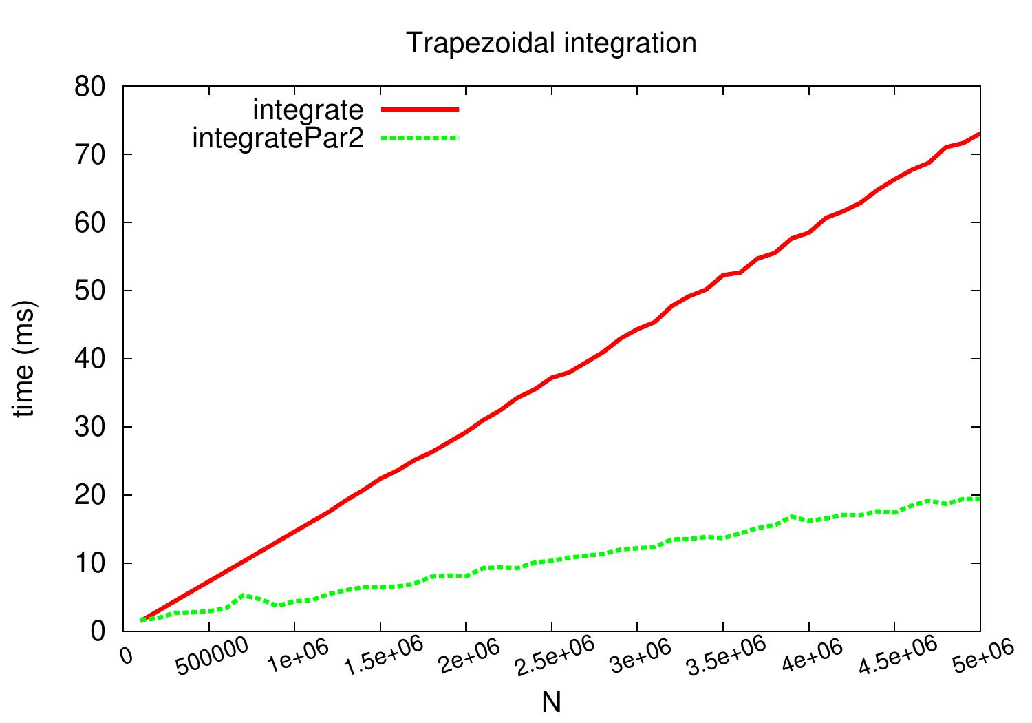
The method integratePar1 is not included in the plot because it is slower than the sequential version: the map method probably builds an intermediate array over which the final sum is then computed. It also has to compute the $ x_k $ and $ f(x_k) $ values twice for each $ k $ while the others are iterative and compute the values only once for most of the indices.

The parallel version integratePar2 obtains a near-linear speedup of roughly 3.7 when $ N = 5 000 000 $.