\(\) \(%\newcommand{\CLRS}{\href{https://mitpress.mit.edu/books/introduction-algorithms}{Cormen et al}}\) \(\newcommand{\CLRS}{\href{https://mitpress.mit.edu/books/introduction-algorithms}{Introduction to Algorithms, 3rd ed.} (\href{http://libproxy.aalto.fi/login?url=http://site.ebrary.com/lib/aalto/Doc?id=10397652}{online via Aalto lib})}\) \(\newcommand{\SW}{\href{http://algs4.cs.princeton.edu/home/}{Algorithms, 4th ed.}}\) \(%\newcommand{\SW}{\href{http://algs4.cs.princeton.edu/home/}{Sedgewick and Wayne}}\) \(\) \(\newcommand{\Java}{\href{http://java.com/en/}{Java}}\) \(\newcommand{\Python}{\href{https://www.python.org/}{Python}}\) \(\newcommand{\CPP}{\href{http://www.cplusplus.com/}{C++}}\) \(\newcommand{\ST}[1]{{\Blue{\textsf{#1}}}}\) \(\newcommand{\PseudoCode}[1]{{\color{blue}\textsf{#1}}}\) \(\) \(%\newcommand{\subheading}[1]{\textbf{\large\color{aaltodgreen}#1}}\) \(\newcommand{\subheading}[1]{\large{\usebeamercolor[fg]{frametitle} #1}}\) \(\) \(\newcommand{\Blue}[1]{{\color{flagblue}#1}}\) \(\newcommand{\Red}[1]{{\color{aaltored}#1}}\) \(\newcommand{\Emph}[1]{\emph{\color{flagblue}#1}}\) \(\) \(\newcommand{\Engl}[1]{({\em engl.}\ #1)}\) \(\) \(\newcommand{\Pointer}{\raisebox{-1ex}{\huge\ding{43}}\ }\) \(\) \(\newcommand{\Set}[1]{\{#1\}}\) \(\newcommand{\Setdef}[2]{\{{#1}\mid{#2}\}}\) \(\newcommand{\PSet}[1]{\mathcal{P}(#1)}\) \(\newcommand{\Card}[1]{{\vert{#1}\vert}}\) \(\newcommand{\Tuple}[1]{(#1)}\) \(\newcommand{\Implies}{\Rightarrow}\) \(\newcommand{\Reals}{\mathbb{R}}\) \(\newcommand{\Seq}[1]{(#1)}\) \(\newcommand{\Arr}[1]{[#1]}\) \(\newcommand{\Floor}[1]{{\lfloor{#1}\rfloor}}\) \(\newcommand{\Ceil}[1]{{\lceil{#1}\rceil}}\) \(\newcommand{\Path}[1]{(#1)}\) \(\) \(%\newcommand{\Lg}{\lg}\) \(\newcommand{\Lg}{\log_2}\) \(\) \(\newcommand{\BigOh}{O}\) \(%\newcommand{\BigOh}{\mathcal{O}}\) \(\newcommand{\Oh}[1]{\BigOh(#1)}\) \(\) \(\newcommand{\todo}[1]{\Red{\textbf{TO DO: #1}}}\) \(\) \(\newcommand{\NULL}{\textsf{null}}\) \(\) \(\newcommand{\Insert}{\ensuremath{\textsc{insert}}}\) \(\newcommand{\Search}{\ensuremath{\textsc{search}}}\) \(\newcommand{\Delete}{\ensuremath{\textsc{delete}}}\) \(\newcommand{\Remove}{\ensuremath{\textsc{remove}}}\) \(\) \(\newcommand{\Parent}[1]{\mathop{parent}(#1)}\) \(\) \(\newcommand{\ALengthOf}[1]{{#1}.\textit{length}}\) \(\) \(\newcommand{\TRootOf}[1]{{#1}.\textit{root}}\) \(\newcommand{\TLChildOf}[1]{{#1}.\textit{leftChild}}\) \(\newcommand{\TRChildOf}[1]{{#1}.\textit{rightChild}}\) \(\newcommand{\TNode}{x}\) \(\newcommand{\TNodeI}{y}\) \(\newcommand{\TKeyOf}[1]{{#1}.\textit{key}}\) \(\) \(\newcommand{\PEnqueue}[2]{{#1}.\textsf{enqueue}(#2)}\) \(\newcommand{\PDequeue}[1]{{#1}.\textsf{dequeue}()}\) \(\) \(\newcommand{\Def}{\mathrel{:=}}\) \(\) \(\newcommand{\Eq}{\mathrel{=}}\) \(\newcommand{\Asgn}{\mathrel{\leftarrow}}\) \(%\newcommand{\Asgn}{\mathrel{:=}}\) \(\) \(%\) \(% Heaps\) \(%\) \(\newcommand{\Downheap}{\textsc{downheap}}\) \(\newcommand{\Upheap}{\textsc{upheap}}\) \(\newcommand{\Makeheap}{\textsc{makeheap}}\) \(\) \(%\) \(% Dynamic sets\) \(%\) \(\newcommand{\SInsert}[1]{\textsc{insert}(#1)}\) \(\newcommand{\SSearch}[1]{\textsc{search}(#1)}\) \(\newcommand{\SDelete}[1]{\textsc{delete}(#1)}\) \(\newcommand{\SMin}{\textsc{min}()}\) \(\newcommand{\SMax}{\textsc{max}()}\) \(\newcommand{\SPredecessor}[1]{\textsc{predecessor}(#1)}\) \(\newcommand{\SSuccessor}[1]{\textsc{successor}(#1)}\) \(\) \(%\) \(% Union-find\) \(%\) \(\newcommand{\UFMS}[1]{\textsc{make-set}(#1)}\) \(\newcommand{\UFFS}[1]{\textsc{find-set}(#1)}\) \(\newcommand{\UFCompress}[1]{\textsc{find-and-compress}(#1)}\) \(\newcommand{\UFUnion}[2]{\textsc{union}(#1,#2)}\) \(\) \(\) \(%\) \(% Graphs\) \(%\) \(\newcommand{\Verts}{V}\) \(\newcommand{\Vtx}{v}\) \(\newcommand{\VtxA}{v_1}\) \(\newcommand{\VtxB}{v_2}\) \(\newcommand{\VertsA}{V_\textup{A}}\) \(\newcommand{\VertsB}{V_\textup{B}}\) \(\newcommand{\Edges}{E}\) \(\newcommand{\Edge}{e}\) \(\newcommand{\NofV}{\Card{V}}\) \(\newcommand{\NofE}{\Card{E}}\) \(\newcommand{\Graph}{G}\) \(\) \(\newcommand{\SCC}{C}\) \(\newcommand{\GraphSCC}{G^\text{SCC}}\) \(\newcommand{\VertsSCC}{V^\text{SCC}}\) \(\newcommand{\EdgesSCC}{E^\text{SCC}}\) \(\) \(\newcommand{\GraphT}{G^\text{T}}\) \(%\newcommand{\VertsT}{V^\textup{T}}\) \(\newcommand{\EdgesT}{E^\text{T}}\) \(\) \(%\) \(% NP-completeness etc\) \(%\) \(\newcommand{\Poly}{\textbf{P}}\) \(\newcommand{\NP}{\textbf{NP}}\) \(\newcommand{\PSPACE}{\textbf{PSPACE}}\) \(\newcommand{\EXPTIME}{\textbf{EXPTIME}}\)

Introduction

The clock speed and processing power of a single computing core are not increasing anymore in the rate they used do in the past. Instead, increasing computing power is obtained by having more computing units running in parallel. This change in the computing environment requires algorithms to be modified to work in such a setting if one wants to use all the resources provided.

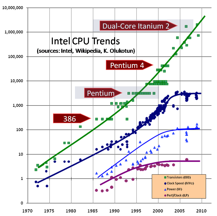
The classic figure below (source: H. Sutter, DDJ) shows how the clock speeds of CPUs stopped growing exponentially while the numbers of transistors in them kept increasing.

_images/CPU.png

A more recent figure below (source: Max Rosser, OurWorldInData.org) shows that Moore’s law, telling that the number of transistor in a chip increases exponentially, has been holding at least until 2018:

_images/Transistor-Count-over-time-to-2018.png

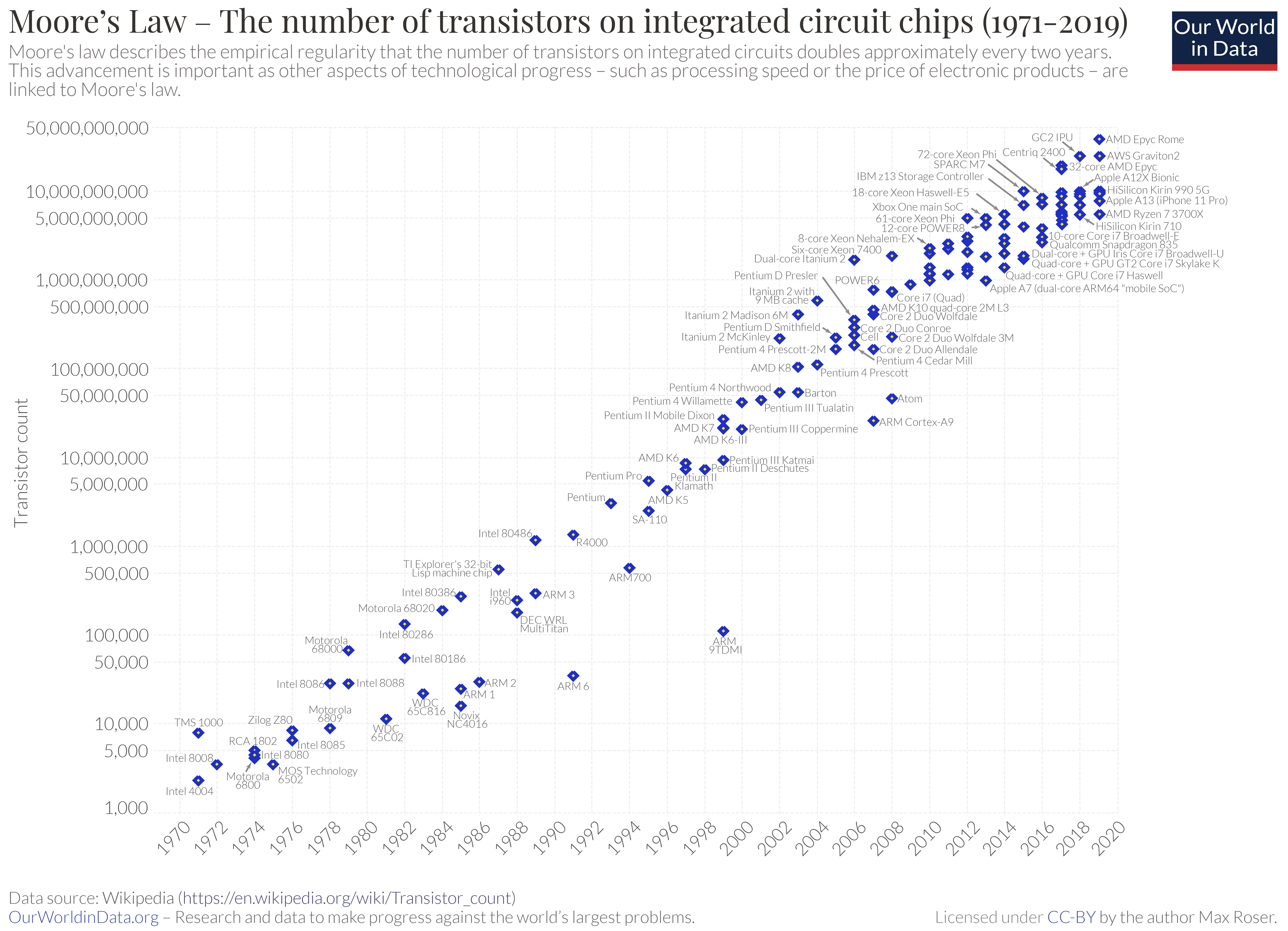
As mentioned above, the increasing number of transistors has been used to having more computing units in a chip. This means that the programmers must change their algorithms and software so that they can use the parallel resources provided; see, for instance, this video by Intel explaining why “software free lunch” is over, meaning that the software developers cannot simply wait for faster chips but have to consider how to parallelize their code.

Multicore processors

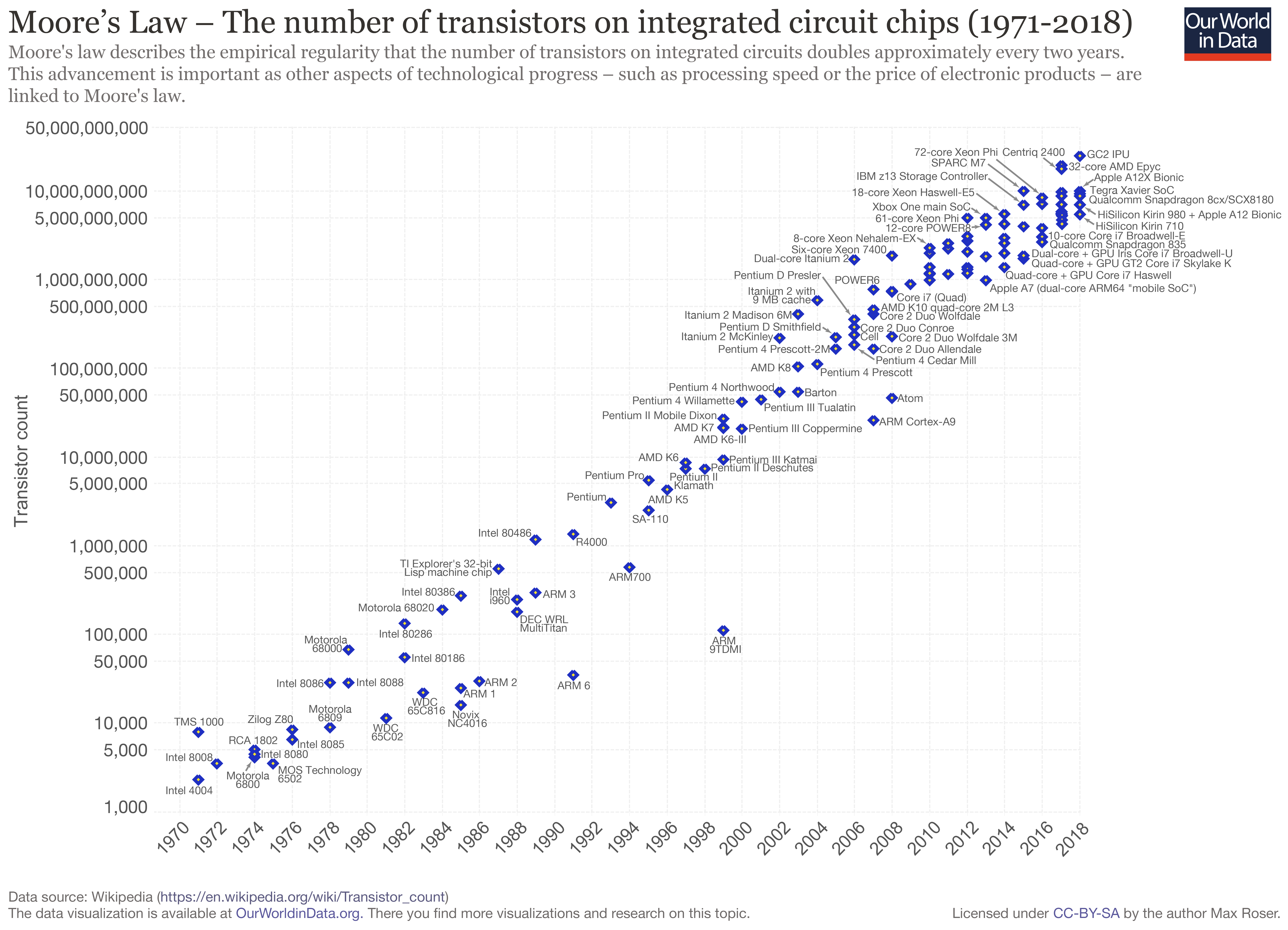
In this round, we will focus on multithreaded algorithms run in multicore machines. In such machines, like standard desktop PCs and modern laptops, the processor contains multiple computing units, called CPU “cores”, running in parallel. The cores can communicate through shared memory. As an example, the figure below shows that architecture of a 12-core Intel processor (source: Intel 64 and IA-32 Architectures Optimization Reference Manual).

_images/Haswell.png

In this setting, code is run in parallel in different threads that have shared memory. Even in this setting, there are different levels of abstraction such as:

  • ​ Programming with threads directly (using locks, semaphores etc to synchronize).

  • ​ Using a concurrency platform. For instance, in the fork-join framework threads in a thread pool execute tasks in parallel.

  • ​ Using a parallel collections library such as Scala parallel collections.

  • ​ Using futures and promises.

In this course, we focus on the fork-join framework and see how they can be used to define methods in a parallel collections library. In fact, the Java fork-join framework, that we will use, is also used to implement the scala.collection.parallel library (documentation). In addition, we see how some algorithms, such as mergesort and other sorting algorithms, can be parallelized in the fork-join framework.

Other parallel hardware systems

Multicore processors are only one kind of computing environment exhibiting parallelism.

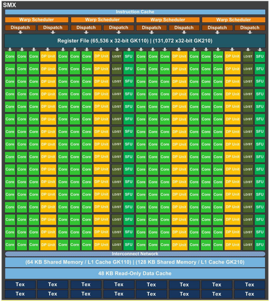
The general-purpose graphics processing units, GPUs, have even a larger amount of cores in a chip. As an example, the figure below shows the architecture of the Kepler GK110/GK210 GPU having 192 cores and some other special units (source: NVIDIA Kepler TM GK110/210 whitepaper). Programming such GPUs is somewhat different to that of multicore processors: they typically use the single instruction, multiple threads (SIMT) paradigm, where a set of threads is executed in a synchronized manner. For low-level programming, one can use the CUDA or OpenCL programming platforms. Of course, one can also use thrust or some other libraries provided by NVIDIA and others.

_images/GPU.png

On the other end of the spectrum, computing clusters and data centers offer a large number of computers that are connected through high-speed connections. As an example, below is a picture of a Google data center (source: google gallery). Again, programming such environment is different to programming multicore processors and one can use Apache spark engine, MapReduce programming model, OpenMP and so on. One can see, for instance, the following online book:

_images/Oklahoma.jpg

More about different forms of parallelism are discussed in the following Aalto courses:

  • CS-E4580 Programming Parallel Computers (5cr, period V): more about programming multicore machines and GPUs

  • ​ CS-E4110 Concurrent programming (5cr, periods I and II): memory models, synchronization primitives, concurrency theory, actors, debugging

  • ​ CS-E4640 Big Data Platforms (5cr, periods I and II): cloud computing technologies

  • ​ CS-E4510 Distributed Algorithms (5cr, periods I and II): algorithms that are distributed to several machines and exchange messages in order to compute the final result