Parallel mergesort¶

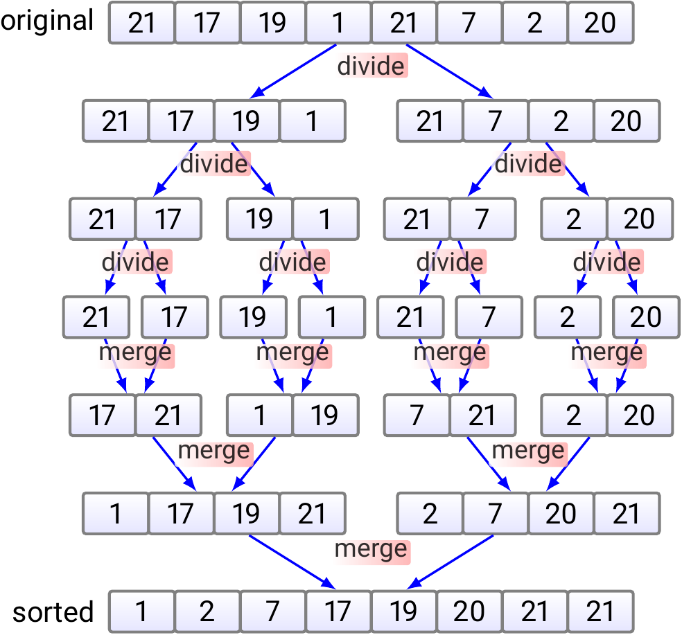
As another example of parallelizing algorithms in Fork-join framework, let’s make parallel versions of the Mergesort algorithm. We’ll build two version with varying amount of parallelism. But first, let’s recap the idea of sequential mergesort. As explained earlier, mergesort splits the array to be sorted into smaller sub-arrays until the sub-arrays become of size 1 and thus sorted. The smaller already sorted sub-arrays are then merged together so that the merged sub-array is also sorted. The high-level idea was illustrated in the following figure.

An implementation of the “merge” operation in Scala is:

object mergesort {
  def merge(a: Array[Int], aux: Array[Int],
            start: Int, mid: Int, end: Int): Unit = {
    var (i, j, dest) = (start, mid, start)
    while (i < mid && j <= end) { // Merge to aux, smallest first
      if (a(i) <= a(j)) { aux(dest) = a(i); i += 1 }
      else { aux(dest) = a(j); j += 1 }
      dest += 1
    }
    while (i < mid) { aux(dest) = a(i); i += 1; dest += 1 }  //Copy rest
    while (j <= end) { aux(dest) = a(j); j += 1; dest += 1 } //Copy rest
    dest = start // Copy from aux back to a
    while (dest <= end) { a(dest) = aux(dest); dest += 1 }
  }
  ...
}

The running time of the merge operation is $ \Theta(k) $, where $ k $ is the size of the two consecutive sub-arrays. When small sub-arrays are sorted with insertion sort (this is a practical optimization to avoid recursion into too small sub-arrays where the recursion takes more time than the merging), the main method of mergesort in Scala can be written as

object mergesort {
  def merge(a: Array[Int], aux: Array[Int],
            start: Int, mid: Int, end: Int): Unit = ...

  /** Sort the array with the merge sort algorithm */
  def sort(a: Array[Int], threshold: Int = 64): Unit = {
    if (a.length <= 1) return
    val aux = new Array[Int](a.length)
    def _mergesort(start: Int, end: Int): Unit = {
      if (start >= end) return
      if(end - start < threshold) insertionsort.sort(a, start, end)
      else {
	val mid = start + (end - start) / 2
	_mergesort(start, mid)
	_mergesort(mid + 1, end)
	merge(a, aux, start, mid + 1, end)
      }
    }
    _mergesort(0, a.length - 1)
  }
}

The first version¶

In the first parallel version, we simply perform the (recursive) sorting of the left and right halves of a sub-array in parallel. In pseudo-code:

Merge-sort-par1(\( A \), \( l \), \( r \)):
  if \( l < r \):
    \( m = l + \Floor{(r-l)/2} \) // The midpoint
    spawn Merge-sort-par1(\( A \), \( l \), \( m \))
    Merge-sort-par1(\( A \), \( m+1 \), \( r \))
    sync
    Merge(\( A \), \( l \), \( m \), \( r \)) // Merge the sorted subarrays \( A[l,m] \) and \( A[m+1,r] \)
 

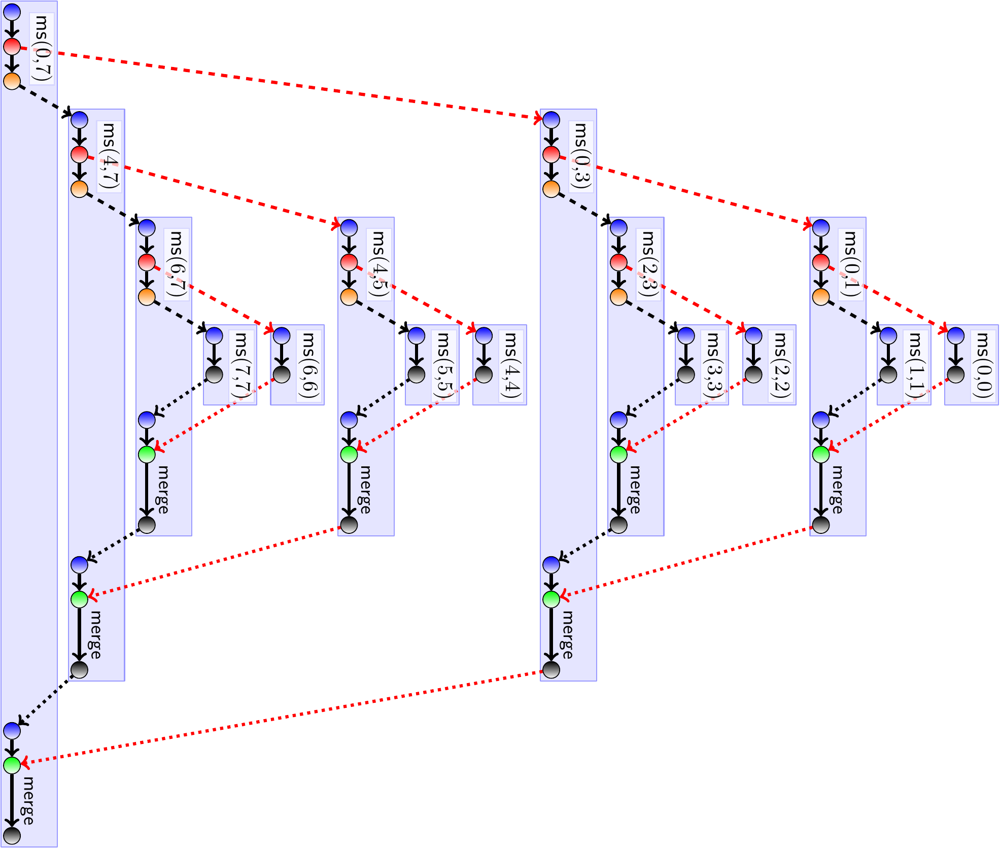
Notice that this is a simplified version, not including special handling of small sub-arrays etc. The following figure illustrates the methods calls, spawns, syncs and merge operations done in a small example array of size 8. The meanings for the nodes are:

blue $ \sim $ method entry
red $ \sim $ “spawn”
orange $ \sim $ method call
green $ \sim $ “sync”
black $ \sim $ return

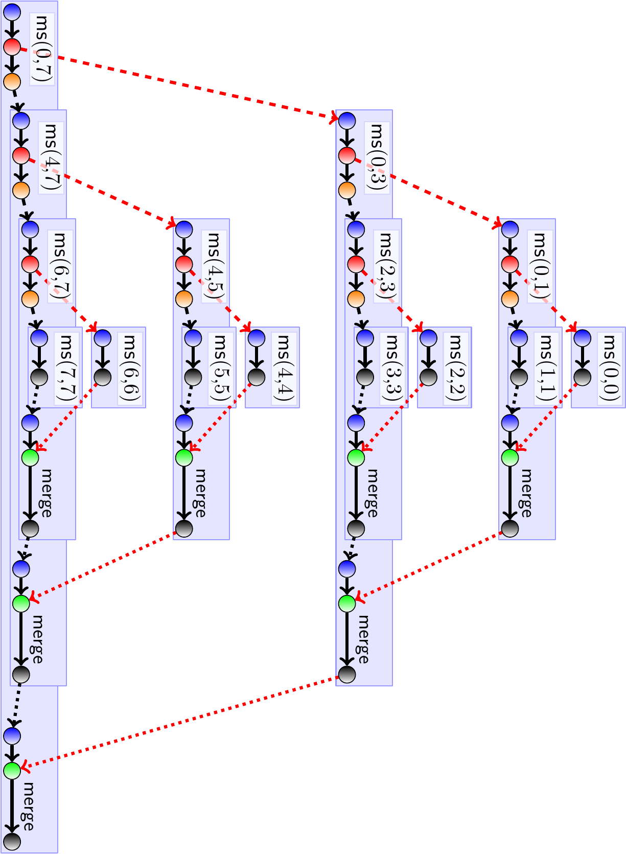
Below is the same figure but the method calls executed in the same thread are drawn on top of the calling method. Here we assume an unlimited amount of available threads.

Experimental evaluation¶

Implementing the first parallel version in Scala is almost trivial by using the sequential version and the par.parallel construction:

object mergesort {
  ...

  /** Sort the array with a simple parallel merge sort algorithm */
  def sortPar(a: Array[Int], threshold: Int = 64): Unit = {
    if (a.length <= 1) return
    val aux = new Array[Int](a.length)
    def _mergesort(start: Int, end: Int): Unit = {
      if (start >= end) return
      if(end - start < threshold) insertionsort.sort(a, start, end)
      else {
        val mid = start + (end - start) / 2
        par.parallel(  // THE ONLY CHANGE IS HERE!
          _mergesort(start, mid),
          _mergesort(mid + 1, end)
        )
        merge(a, aux, start, mid + 1, end)
      }
    }
    _mergesort(0, a.length - 1)
  }
}

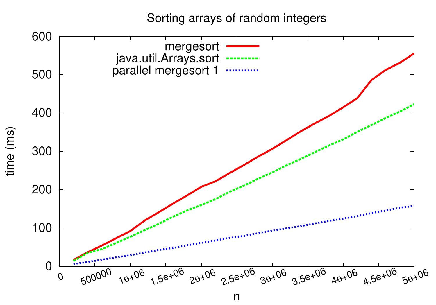
How well does this work in practice? The plot below shows wall-clock running times when the code is run on a Linux Ubuntu 16.04 machine with Intel Xeon E31230 quad-core CPU running at 3.2GHz. As we can see, compared to the sequential version, we obtain speedup of $ \approx 3.5 $ on arrays with five million random integers.

Work, span, and parallelism¶

To analyze the work and the span of the simple parallel mergesort, consider again the graphical representation below.

In each computation path, recursive tasks are spawned, synchronized, and then the sorted sub-arrays are merged. The work on each path is roughly the same:

Logarithmic amount of constant-time operations (end condition check, spawn, sync)
The merge of the sub-arrays of lengths $ n $, $ \approx n/2 $, $ \approx n/4 $, and so on. As each merge is a linear time operation, the merges on a path take time $ \Theta(n + n_2 + n_4 + .. + 1) = \Theta(2n) = \Theta(n) $.

Thus the span is $ \Theta(\Lg{n}+n)=\Theta(n) $. The work is the same $ \Theta(n \Lg n) $ as the running time of the sequential version because the only additions are the spawns and syncs but there are as many of them as recursion calls and returns in the sequential version.

We can also form a recurrence for the span:

$ T(0) = T(1) = d $
$ T(n) = d + \max\Set{T(\Floor{n/2}),T(\Ceil{n/2})} + cn $, where $ c $ and $ d $ are some constants

Assuming that $ n = 2^k $ for some $ k $, we get $ T(2^k) = d + T(2^k/2) + c2^k $ and can “telescope” this into \begin{eqnarray*} T(2^k) &=& d + c2^k + T(2^k/2)\\ &=& d + c2^k + (d + c2^{k-1} + T(2^{k-1}/2))\\ &=& … \\ &=& dk + c(2^{k+1}-2) \end{eqnarray*} because $ 2^k + 2^{k-1} + … + 2^{k-(k-1)} = 2^{k+1}-2 $. Thus $ T(n) = \Oh{\Lg{n} + n} = \Oh{n} $.

That is: no matter how many processors one has, the algorithm still takes linear time. Note that in Java and Scala the auxiliary array is (unnecessarily) initialized, taking already $ \Oh{n} $ time. We defined the amount of parallelism to be $$\frac{\text{work}}{\text{span}}$$ In this algorithm, it is quite modest $ \Oh{\Lg{n}} $. Thus, although the experimental results on a multi-core machine with few cores looks good, the theoretical limit for the scalability for machines with a lot of cores is not very good. Inspecting the figure and the analysis, it is quite easy to spot the tasks with the highest amount of work: the sequential merges at the end of each computation path.

The second version: parallelizing the merge operation¶

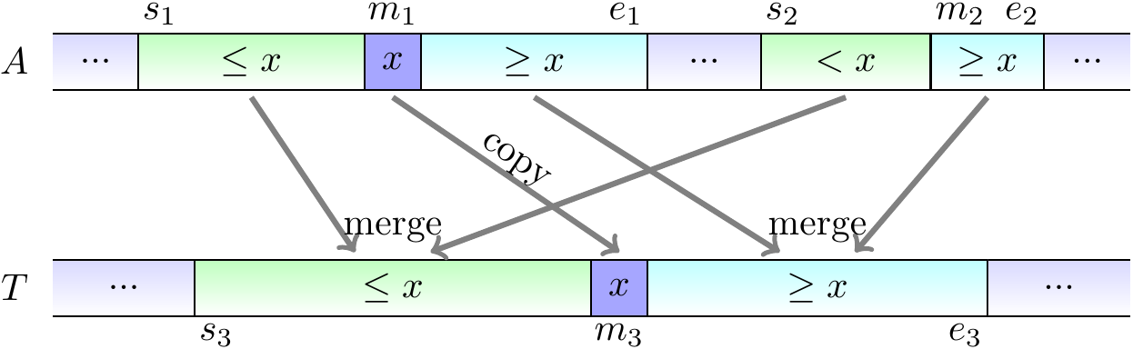
To improve the parallelism of mergesort, we can parallelize the merge operation as well. Although merging two sorted sub-arrays seems an inherently sequential operation at first, it can also be parallelized with a divide-and-conquer approach. The idea in merging two disjoint sorted sub-arrays $ A_1 = A[s_1,e_1] $ and $ A_2 = A[s_2,e_2] $ to a temporary sub-array $ T[s_3,e_3] $ with $ e_3-s_3= (e_1-s_1)+(e_2-s_2) $ is to

take the larger sorted sub-array, say $ A_1 = A[s_1,e_1] $, and find its middle index $ m_1 $ and element $ x = A[m_1] $,
find (with binary search) the index $ m_2 $ in the smaller sub-array $ A_2 = A[s_2,e_2] $ such that
- all the elements in $ A[s_2,m_2-1] $ are less than $ x $ and
- all the elements in $ A[m_2,e_2] $ are at least $ x $
copy $ x $ to its position $ T[m_3] $, where $ m_3 = s_3 + (m_1-s_1) + (m_2-s_2) $
merge recursively and in parallel
- the sub-arrays $ A[s_1,m_1-1] $ and $ A[s_2,m_2-1] $ to $ T[s_3,m_3-1] $, and
- the sub-arrays $ A[m_1+1,e_2] $ and $ A[m_2,e_2] $ to $ T[m_3+1,e_3] $.

The first three steps above can be illustrated by the following figure. Observe that here the sub-arrays $ A[s_1,e_1] $ and $ A[s_2,e_2] $ are not always consecutive anymore.

In pseudo-code, we can express the parallel merge operation as follows:

Merge-par(\( A \), \( s_1 \), \( e_1 \), \( s_2 \), \( e_2 \), \( T \), \( s_3 \)):
  \( l_1 \Asgn e_1 - s_1 \) // The lenght of the "left" part
  \( l_2 \Asgn e_2 - s_2 \) // The lenght of the "right" part
  if \( l_1 < l_2 \): // Ensure the "left" part is of equal size or larger
    swap \( s_1 \) and \( s_2 \)
    swap \( e_1 \) and \( e_2 \)
    swap \( l_1 \) and \( l_2 \)
  if \( l_1 = 0 \): // Both parts empty?
    return
  else:
    \( m_1 \Asgn \Floor{s_1 + l_1/2} \) // Midpoint in the "left" part
    \( m_2 \Asgn {} \)Binary-search(\( A[m_1] \), \( A \), \( s_2 \), \( e_2 \)) // Split point in the "right" part
    \( m_3 \Asgn s_3 + (m_1 - s_1) + (m_2 - s_2) \) // Midpoint in the merged result
    \( T[m_3] \Asgn A[m_1] \)
    spawn Merge-par(\( A \), \( s_1 \), \( m_1-1 \), \( s_2 \), \( m_2-1 \), \( T \), \( s_3 \))
    Merge-par(\( A \), \( m_1+1 \), \( e_1 \), \( m_2 \), \( e_2 \), \( T \), \( m_3+1 \))
    sync
 

The applied version of the binary search is:

Binary-search(\( value \), \( A \), \( s \), \( e \)):
  \( low \Asgn s \)
  \( high \Asgn \max\Set{s, e+1} \)
  while \( low < high \):
    \( mid \Asgn \Floor{(low + high)/2} \)
    if \( value \le A[mid] \): \( high \Asgn mid \)
    else: \( low \Asgn mid+1 \)
  return \( high \)
 

Implementation in Scala is left as a programming exercise. In a real implementation, one should again handle small sub-arrays sequentially.

Work of parallel merge is $ \Theta(k) $ and the span is $ \Oh{\Lg^2 k} $, where $ k $ is the length of the merged sub-arrays (analysis is given in the book Introduction to Algorithms, 3rd ed. (online via Aalto lib) but it is not required in this course).

The pseudo-code for our parallel mergesort with a parallel merge operation is as follows:

Mergesort-par(\( A \)):
  let \( aux \) be a new array of length \( \ALengthOf{A} \)
  def inner(\( from \), \( to \), \( s \), \( e \)):
    if \( e-s < k \): // k is some small constant (32?) for "small sub-arrays"
      if \( A \neq to \):
        copy \( A[s,e] \) to \( to[s,e] \)
      insertion-sort(\( to \), \( s \), \( e \))
    else:
      \( m = \Floor{s + (e-s)/2} \)
      spawn inner(\( to \), \( from \), \( s \), \( m \))
      inner(\( to \), \( from \), \( m+1 \), \( e \))
      sync
      merge-par(\( from \), \( s \), \( m \), \( m+1 \), \( e \), \( to \), \( s \))
  inner(\( aux \), \( A \), \( 1 \), \( \ALengthOf{A} \))
 

Note the optimization swapping the original and auxiliary array references in the recursive calls to the inner function; in this way, there is no need to copy data back from the auxiliary array $ aux $ to the original array $ A $ inside the merge operation.

The book Introduction to Algorithms, 3rd ed. (online via Aalto lib) gives (in Section 27.3, page 804) a “plain” version of the algorithm with no special handling of small sub-arrays but with more auxiliary memory use. For that version,

the work is $ \Oh{n \Lg{n}} $,
the span is $ \Lg^3n $, and
the parallelism is $ \Oh{n / \Lg^2n} $.

The proofs of these are not required in the course.

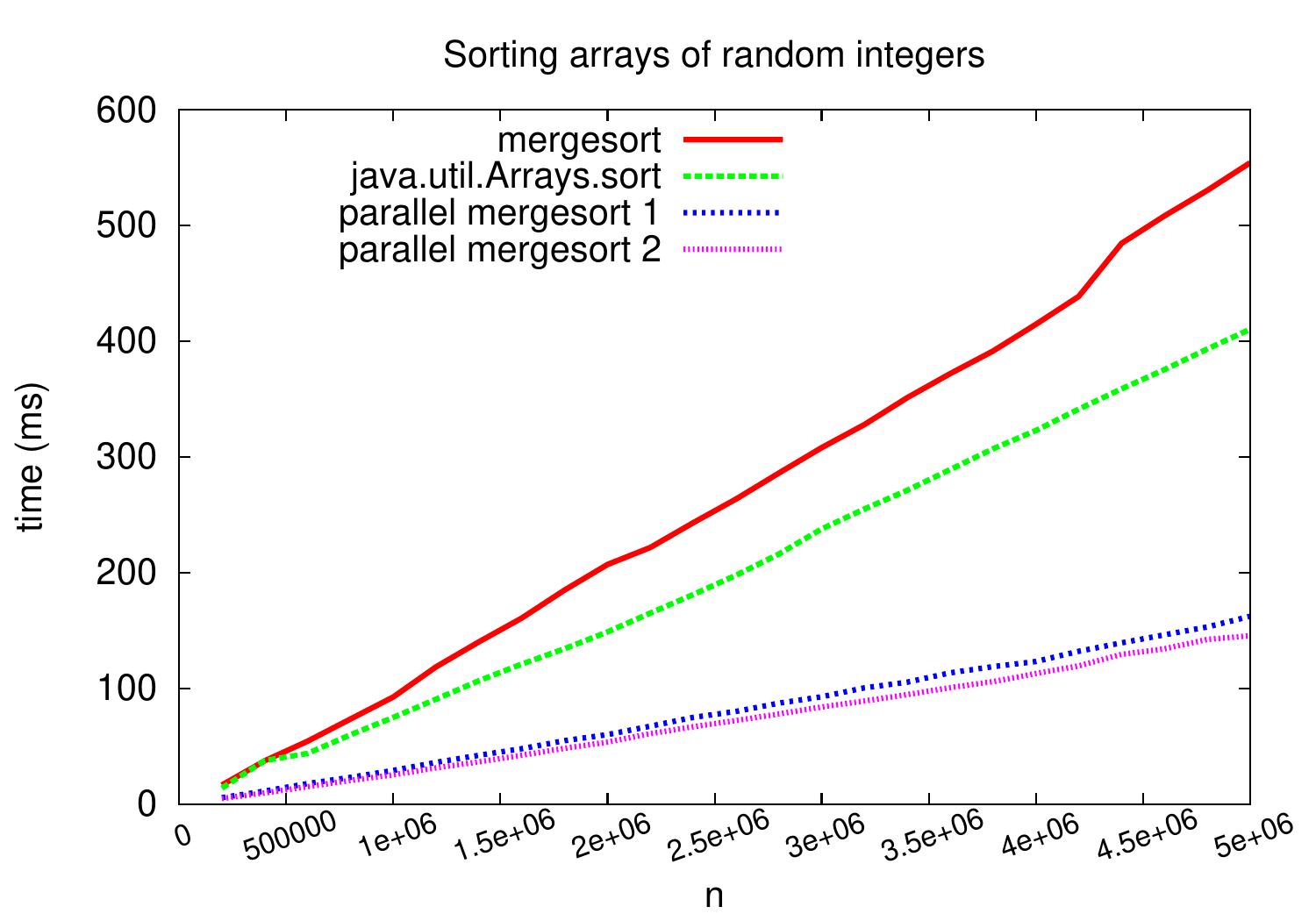
Experimental evaluation¶

The plot below shows a comparison between the first and the second parallel version when used to sort arrays of random integers. As we can see, very modest speedup is obtained compared to the first simple parallel version. This is probably because the memory bus of the computer is the bottleneck in this case: doing the computations inside the merges, i.e., comparing two integers, is quite cheap.

If we perform the same comparison but now with arrays of shortish strings, we obtain speedup of about 1.5 compared to the simple version. In this case the comparisons require more computation and the memory bus is not always the bottleneck.

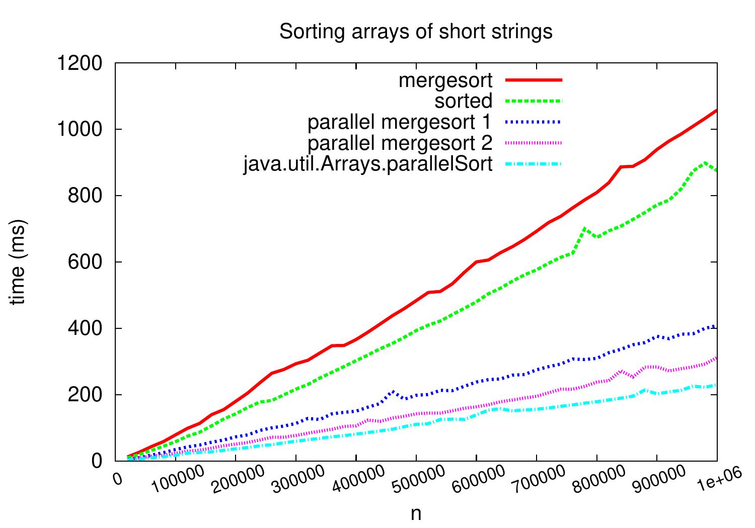
_images/mergesort-parallel-strings-2018.jpg

We also observe that Java’s parallel sort is bit more efficient than our simple parallel mergesort versions. The Java version/implementation that was used in the experiments performs parallel mergesort (with parallel merge) except that for sorting small sub-arrays, it performs either a version of quicksort (for primitive types such as integers) or TimSort (for object types such as strings).