\(\)
\(%\newcommand{\CLRS}{\href{https://mitpress.mit.edu/books/introduction-algorithms}{Cormen et al}}\)
\(\newcommand{\CLRS}{\href{https://mitpress.mit.edu/books/introduction-algorithms}{Introduction to Algorithms, 3rd ed.} (\href{http://libproxy.aalto.fi/login?url=http://site.ebrary.com/lib/aalto/Doc?id=10397652}{online via Aalto lib})}\)
\(\newcommand{\SW}{\href{http://algs4.cs.princeton.edu/home/}{Algorithms, 4th ed.}}\)
\(%\newcommand{\SW}{\href{http://algs4.cs.princeton.edu/home/}{Sedgewick and Wayne}}\)
\(\)
\(\newcommand{\Java}{\href{http://java.com/en/}{Java}}\)
\(\newcommand{\Python}{\href{https://www.python.org/}{Python}}\)
\(\newcommand{\CPP}{\href{http://www.cplusplus.com/}{C++}}\)
\(\newcommand{\ST}[1]{{\Blue{\textsf{#1}}}}\)
\(\newcommand{\PseudoCode}[1]{{\color{blue}\textsf{#1}}}\)
\(\)
\(%\newcommand{\subheading}[1]{\textbf{\large\color{aaltodgreen}#1}}\)
\(\newcommand{\subheading}[1]{\large{\usebeamercolor[fg]{frametitle} #1}}\)
\(\)
\(\newcommand{\Blue}[1]{{\color{flagblue}#1}}\)
\(\newcommand{\Red}[1]{{\color{aaltored}#1}}\)
\(\newcommand{\Emph}[1]{\emph{\color{flagblue}#1}}\)
\(\)
\(\newcommand{\Engl}[1]{({\em engl.}\ #1)}\)
\(\)
\(\newcommand{\Pointer}{\raisebox{-1ex}{\huge\ding{43}}\ }\)
\(\)
\(\newcommand{\Set}[1]{\{#1\}}\)
\(\newcommand{\Setdef}[2]{\{{#1}\mid{#2}\}}\)
\(\newcommand{\PSet}[1]{\mathcal{P}(#1)}\)
\(\newcommand{\Card}[1]{{\vert{#1}\vert}}\)
\(\newcommand{\Tuple}[1]{(#1)}\)
\(\newcommand{\Implies}{\Rightarrow}\)
\(\newcommand{\Reals}{\mathbb{R}}\)
\(\newcommand{\Seq}[1]{(#1)}\)
\(\newcommand{\Arr}[1]{[#1]}\)
\(\newcommand{\Floor}[1]{{\lfloor{#1}\rfloor}}\)
\(\newcommand{\Ceil}[1]{{\lceil{#1}\rceil}}\)
\(\newcommand{\Path}[1]{(#1)}\)
\(\)
\(%\newcommand{\Lg}{\lg}\)
\(\newcommand{\Lg}{\log_2}\)
\(\)
\(\newcommand{\BigOh}{O}\)
\(%\newcommand{\BigOh}{\mathcal{O}}\)
\(\newcommand{\Oh}[1]{\BigOh(#1)}\)
\(\)
\(\newcommand{\todo}[1]{\Red{\textbf{TO DO: #1}}}\)
\(\)
\(\newcommand{\NULL}{\textsf{null}}\)
\(\)
\(\newcommand{\Insert}{\ensuremath{\textsc{insert}}}\)
\(\newcommand{\Search}{\ensuremath{\textsc{search}}}\)
\(\newcommand{\Delete}{\ensuremath{\textsc{delete}}}\)
\(\newcommand{\Remove}{\ensuremath{\textsc{remove}}}\)
\(\)
\(\newcommand{\Parent}[1]{\mathop{parent}(#1)}\)
\(\)
\(\newcommand{\ALengthOf}[1]{{#1}.\textit{length}}\)
\(\)
\(\newcommand{\TRootOf}[1]{{#1}.\textit{root}}\)
\(\newcommand{\TLChildOf}[1]{{#1}.\textit{leftChild}}\)
\(\newcommand{\TRChildOf}[1]{{#1}.\textit{rightChild}}\)
\(\newcommand{\TNode}{x}\)
\(\newcommand{\TNodeI}{y}\)
\(\newcommand{\TKeyOf}[1]{{#1}.\textit{key}}\)
\(\)
\(\newcommand{\PEnqueue}[2]{{#1}.\textsf{enqueue}(#2)}\)
\(\newcommand{\PDequeue}[1]{{#1}.\textsf{dequeue}()}\)
\(\)
\(\newcommand{\Def}{\mathrel{:=}}\)
\(\)
\(\newcommand{\Eq}{\mathrel{=}}\)
\(\newcommand{\Asgn}{\mathrel{\leftarrow}}\)
\(%\newcommand{\Asgn}{\mathrel{:=}}\)
\(\)
\(%\)
\(% Heaps\)
\(%\)
\(\newcommand{\Downheap}{\textsc{downheap}}\)
\(\newcommand{\Upheap}{\textsc{upheap}}\)
\(\newcommand{\Makeheap}{\textsc{makeheap}}\)
\(\)
\(%\)
\(% Dynamic sets\)
\(%\)
\(\newcommand{\SInsert}[1]{\textsc{insert}(#1)}\)
\(\newcommand{\SSearch}[1]{\textsc{search}(#1)}\)
\(\newcommand{\SDelete}[1]{\textsc{delete}(#1)}\)
\(\newcommand{\SMin}{\textsc{min}()}\)
\(\newcommand{\SMax}{\textsc{max}()}\)
\(\newcommand{\SPredecessor}[1]{\textsc{predecessor}(#1)}\)
\(\newcommand{\SSuccessor}[1]{\textsc{successor}(#1)}\)
\(\)
\(%\)
\(% Union-find\)
\(%\)
\(\newcommand{\UFMS}[1]{\textsc{make-set}(#1)}\)
\(\newcommand{\UFFS}[1]{\textsc{find-set}(#1)}\)
\(\newcommand{\UFCompress}[1]{\textsc{find-and-compress}(#1)}\)
\(\newcommand{\UFUnion}[2]{\textsc{union}(#1,#2)}\)
\(\)
\(\)
\(%\)
\(% Graphs\)
\(%\)
\(\newcommand{\Verts}{V}\)
\(\newcommand{\Vtx}{v}\)
\(\newcommand{\VtxA}{v_1}\)
\(\newcommand{\VtxB}{v_2}\)
\(\newcommand{\VertsA}{V_\textup{A}}\)
\(\newcommand{\VertsB}{V_\textup{B}}\)
\(\newcommand{\Edges}{E}\)
\(\newcommand{\Edge}{e}\)
\(\newcommand{\NofV}{\Card{V}}\)
\(\newcommand{\NofE}{\Card{E}}\)
\(\newcommand{\Graph}{G}\)
\(\)
\(\newcommand{\SCC}{C}\)
\(\newcommand{\GraphSCC}{G^\text{SCC}}\)
\(\newcommand{\VertsSCC}{V^\text{SCC}}\)
\(\newcommand{\EdgesSCC}{E^\text{SCC}}\)
\(\)
\(\newcommand{\GraphT}{G^\text{T}}\)
\(%\newcommand{\VertsT}{V^\textup{T}}\)
\(\newcommand{\EdgesT}{E^\text{T}}\)
\(\)
\(%\)
\(% NP-completeness etc\)
\(%\)
\(\newcommand{\Poly}{\textbf{P}}\)
\(\newcommand{\NP}{\textbf{NP}}\)
\(\newcommand{\PSPACE}{\textbf{PSPACE}}\)
\(\newcommand{\EXPTIME}{\textbf{EXPTIME}}\)
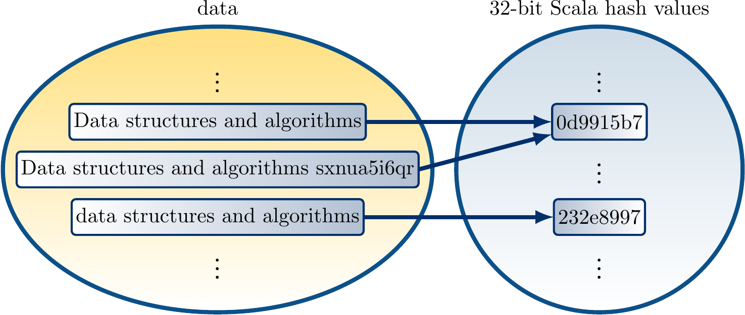
Round 5: Hashing
A hash function is a function that takes some data as input and
produces a fixed-size hash value for the data.
Depending on the application area, the hash values can also be called
“hash codes” or “digests”.
In general, hash functions are used in
In this round, we will focus on the first area and
show how hash tables can be used to implement set and map data structures.
The main difference to the set and map data structures implemented
with balanced binary search trees (recall Section Round 4: Binary Search Trees)
is that the order of the keys is not preserved
in hash table based implementations.
In many applications this does not matter because
sets and maps with only
insert,
search, and
remove
operations are enough and one does not need efficient implementations
for min and successor, for instance.
With hash tables we can perform the insert, search, and remove operations
in \( \Oh{1} \) time on average.
The worst-case time requirement can be \( \Theta(n) \) but with good design this is extremely improbable.
However, finding the smallest and largest elements takes \( \Theta(n) \) time in the worst case and on average.
Some implementations:
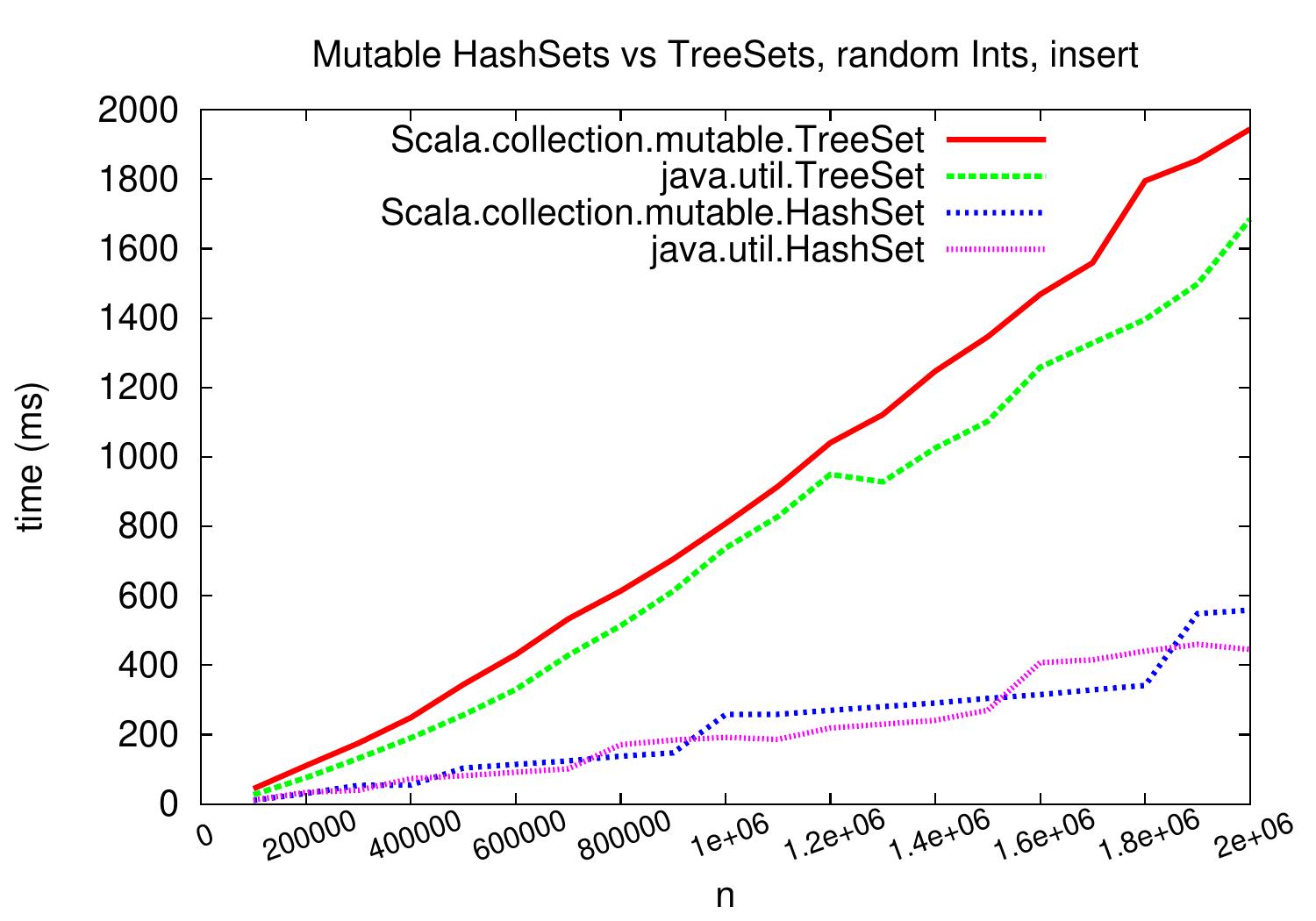
To get a feeling how the performance of hashing based sets, or “hash sets”, relates to
“tree sets” based on balanced binary search trees,
the figure below shows the running times of
inserting up to two million random 32-bit integers into tree and hash sets.
As we can see, hash sets perform better when we do not need to maintain the order between the keys.
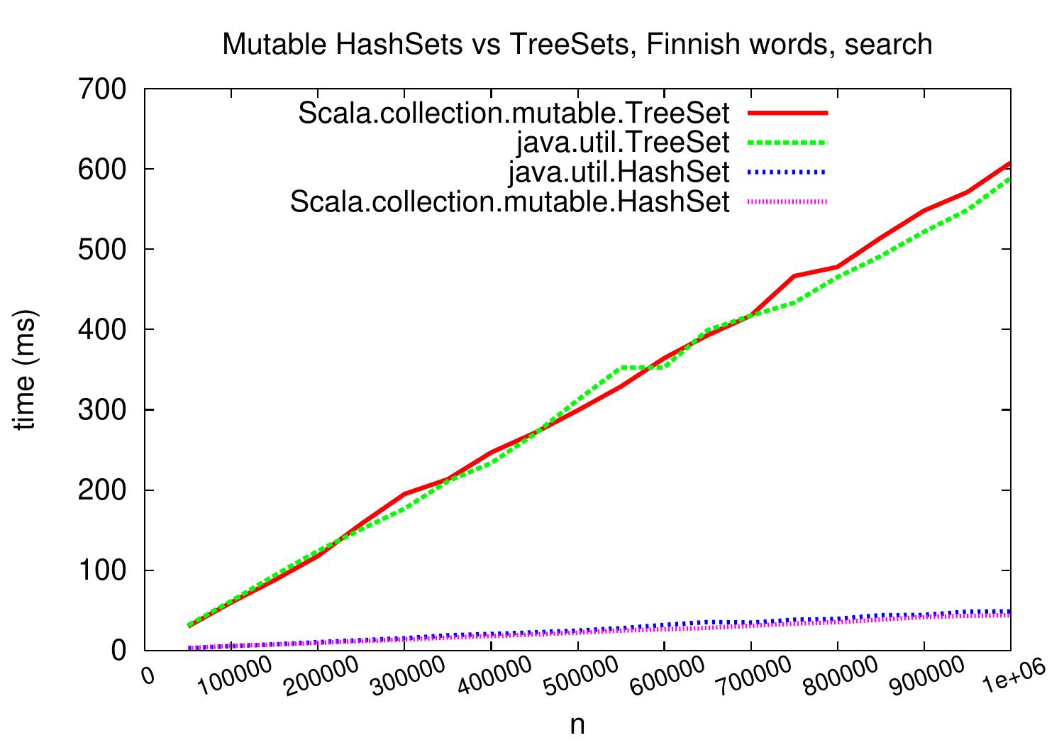
As a second performance comparison between tree and hash sets,
the plot below shows the running times of performing up to
one million successful queries in a set consisting of
roughly 91 thousand Finnish words
(from kotus sanalista).
Again hash sets perform better than tree sets.
Material in the book Introduction to Algorithms, 3rd ed. (online via Aalto lib):
Similar material elsewhere:
Some other external links: