Round 10: Computationally more difficult problems¶

So far almost all of our algorithms have been rather efficient, having worst-case running times such as \( \Oh{\Lg{n}} \), \( \Oh{n} \), \( \Oh{n \Lg{n}} \), \( \Oh{(\NofE + \NofV)\Lg\NofV} \) and so on. But there are lots of (practical!) problems for which we do not know any efficient algorithms. In fact, there are even problems that provably cannot be solved by computers. Here “solve by computers” means “to have an algorithm that in all the cases gives the answer and the answer is correct”. The proof that such problems exists and more about this topic can be found in the Aalto course CS-C2160 Theory of Computation (5cr, periods III-IV).

Example

There is no algorithm that always decides whether a multivariate polynomial has integer-valued roots.

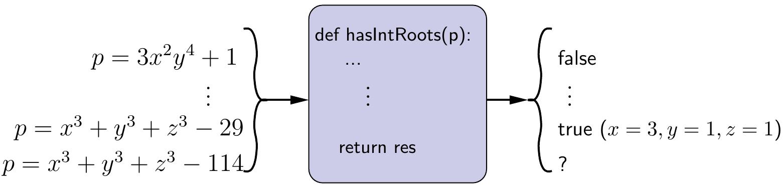
As a curiosity, the output to \( x^3+y^3+z^3-114 \) is marked with “?” in the figure because we do not currently (September 2020) know whether the are integers \( x \), \( y \) and \( z \) such that \( x^3+y^3+z^3 = 114 \). The cases 33 and 42 were solved only in 2019, see this Wikipedia article.

This round

gives a semi-formal description for one important class of computationally hard but still solvable problems, called \( \NP \)-complete problems, and
provides some methods for attacking such problems in practice.

Definitions by using formal languages etc and most of the proofs are not covered, they are discussed more in the Aalto courses

CS-C2160 Theory of Computation, and
CS-E4530 Computational Complexity Theory.

Contents:

Material:

These notes
Chapter 34 in Introduction to Algorithms, 3rd ed. (online via Aalto lib) on the abstraction level of these notes:
- the formal language definitions are not required,
- nor are the proofs that are not in the notes.

Further references:

Sanjeev Arora and Boaz Barak, Computational Complexity: A Modern Approach