Basic definitions¶

In general, we can use parallelism to speed up a computation if we can divide the computation in tasks that are

independent of each other so that
they can be computed in any order or at the same time.

Definition

Two parallel tasks are independent if the mutable data structures (variables, array elements, mutable lists, output console etc) written by one task are not read or written by the other.

Independence thus guarantees that both tasks will read the same values irrespective of the order they are executed in because the other task cannot write any value read by the other. Similarly, the values written by a task cannot be overwritten by an independent task. As a result, independent tasks can be executed in any order, or at the same time, and the end result is the same.

Example

Suppose that we want to

initialize an array $ A[1,n] $ of $ n $ elements with values so that $ A[i] = f(i) $ for some side-effect free function $ f $, and
then output the array to the console.

If we have multiple cores in use, then:

The first phase can be performed in parallel, each core computing the values $ f(i) $ for some different values of $ i $. This is possible because the side-effect free function computations are independent with respect to each other and the results are written to different indices of the array.
The second phase cannot be parallelized because we want the values to be printed in the correct order. Printing the $ i $th and $ j $th array index are not independent tasks because they write to the same console.

Suppose that a single core can compute the first phase in time $ A $ and the second in time $ B $. Thus the sequential running time is $$T_1 = A + B$$ If we have $ P $ cores in use, the running time is $$T_P = A/P + B$$ The (theoretical) speedup with $ P $ cores is thus $$S_P = \frac{T_1}{T_P} = \frac{A + B}{A/P + B}$$ As an example, if $ A = 12 $, $ B=2 $ and $ P=4 $, then the sequential running time is $ T_1 = 14 $ and the running time with 4 cores is $ T_4 = 5 $. Thus the speedup is $ 2.8 $. In practice the speedup is probably less because launching parallel computations cause overhead etc.

Amdahl’s law¶

In general, suppose that

the running time of a program is $ T_P $ when $ P $ cores are used, and
a portion $ r \in [0,1] $ of the computation can be parallelized.

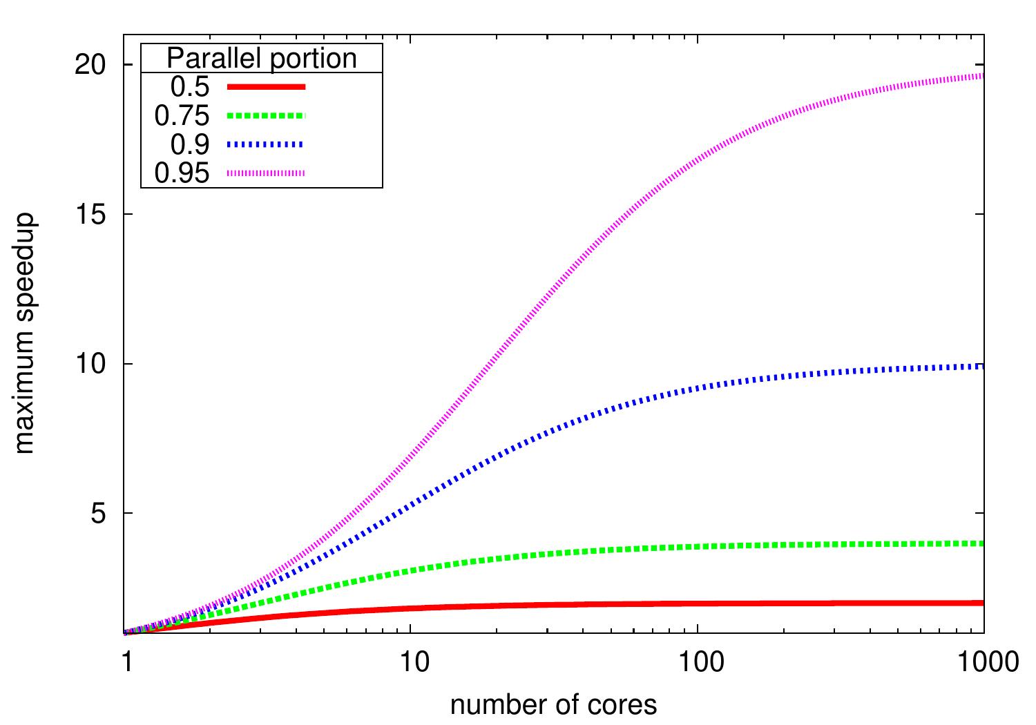
In such a case, $$T_P \ge (1-r)T_1 + rT_1/P$$ where the term $ (1-r)T_1 $ is the running time of the portion that cannot be parallelized, and $ rT_1/P $ is the running time of the parallelizable portion when run on $ P $ cores. The maximum speedup obtained by using $ P $ cores instead of only one is thus at most $$S_P = \frac{T_1}{T_P} \le \frac{T_1}{(1-r)T_1+rT_1/P} = \frac{P}{(1-r)P + r}$$ This is known as Amdahl’s law. In the ideal case with an unbounded amount of cores, $ P $ approaches $ \infty $ and thus the upper bound for the speedup is $ \frac{1}{1-r} $. Thus if 95 percent of the program parallelizes, the maximum speedup is $ 20 $.

Work and span¶

Amdahl’s law discussed above considers a single computation but does not tell us how well an algorithm parallelizes with respect to the problem instance input size $ n $. For this, we extend our earlier running time analysis with the following definitions. In the analysis, we’ll again use the $ \BigOh $-notation and its variants. For a parallel program,

the work $ T_1 $ is its running time on a single core, i.e., the amount of computation done in the whole program, and
the span $ T_{\infty} $ is its running time on an unbounded amount of cores.

Data races¶

Informally, a data race occurs when a thread (running a task) writes to a shared structure that can be read or written by another thread at the same time. Thus, by definition, independent tasks do not contain data races. For the precise definition of data races in Java/Scala, see the Java 8 memory model specification. However, the main thing to observe is:

When code contains a data race, counter-intuitive results are often possible. (From the Java 8 memory model specification.)

Example

Let (i) A and B be shared variables initialized to 0, and (ii) r1 and r2 be thread local variables (registers). Consider the following simple program with two threads:

thread 1	thread 2
a1: `r1 = A`	b1: `r2 = B`
a2: `B = 2`	b2: `A = 1`

There is a data race: the thread 1 writes to B which is read by the thread 2. As a consequence, the final values of the registers r1 and r2 depend on the execution order of the instructions:

The execution order a1,a2,b1,b2 gives r1 == 0 and r2 == 2 at the end
The execution order a1,b1,b2,a2 gives r1 == 0 and r2 == 0
The execution order b1,b2,a1,a2 gives r1 == 1 and r2 == 0

Observe that no execution order, respecting the instruction order within each thread, can give r1 == 1 and r2 == 2 at the end. However, under the Java memory model, it is possible that r1 == 1 and r2 == 2 at the end! The reason is that the compiler or processor may reorder, for performance reasons, the lines r1 = A and B = 2 as their execution order does not matter for the thread 1: if thread 1 would be run in isolation, the result stays the same regardless of the execution order of its two instructions. The Java memory model does not prohibit this kind of reordering. The result corresponds to the program:

thread 1	thread 2
a2. `B = 2`	b1. `r2 = B`
a1. `r1 = A`	b2. `A = 1`

Now the execution order a2,b1,b2,a1 results in r1 == 1 and r2 == 2 at the end.

To ensure that another thread observe the changes made by a thread in correct order, one should use synchronization primitives. More about this in the Aalto course “CS-E4110 Concurrent programming”. For the rest of this round, we aim to build parallel programs that (i) do not have data races and (ii) the synchronization of the threads is handled by an underlying concurrency platform.

Atomicity¶

An operation is atomic if it always appears to have happened completely or not at all. That is, the operation cannot be interrupted in the middle of it and no other thread can observe the intermediate state(s) of the operation. Consider a simple example:

scala> val a = (1 to 10000).toArray
a: Array[Int] = Array(1, 2, 3, 4, 5, 6, 7, 8, ...
scala> var count = 0
scala> count = 0; (0 until a.length).foreach(i => {if((a(i) % 7) == 0) count += 1})
count: Int = 1428
scala> count = 0; (0 until a.length).par.foreach(i => {if((a(i) % 7) == 0) count += 1})
count: Int = 1360

The first foreach line computes the sequential reference value. An erroneous value is produced in the par.foreach line executing the loop body code if((a(i) % 7) == 0) count += 1 in parallel for different values if i because

the loop bodies are not independent as they all write to count, causing a data race, and
the statement count += 1 is not atomic but comprises three atomic instructions:
- read the value of count into a register,
- increment the value of the register by one, and
- write the value in the register back to the shared variable count.
As a consequence, two such statements running in parallel can read the same old value of count, increase their own local values by one, and write the new value to count. The value written first is overwritten by the latter (and thus lost) and the end-result is incorrect.

Many standard libraries, such as java.util.concurrent.atomic and the C++ atomic, provide atomic versions of some data types.

Some notes¶

The following two concepts are needed when we discuss computational tasks than can execute in different computing units.

Concurrency: multiple tasks can happen at the same time. It is possible to have concurrent programs running in a single core: the threads are executed in time-sharing slices.
Parallelism: multiple tasks are actually active at the same time.

For more discussion about the concepts, please see the Wikipedia pages of concurrent programming and parallel programming.