Naive matrix multiplication
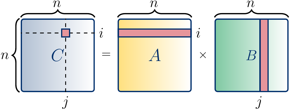
Let’s again recall the matrix multiplication example from the CS-A1120 Programming 2 course. The product of two \( n \times n \) matrices \( A = (a_{i,j}) \) and \( B = (b_{i,j}) \) is the \( n \times n \) matrix \( C = (c_{i,j}) \) where $$c_{i,j} = \sum_{k=1}^n a_{i,k}b_{k,j}$$ The figure below shows, in red, the entries involved in the computation of the entry \( c_{ij} \) in the product matrix \( C \).
Computing the product matrix by using this formulation is an embarrassingly parallel problem as the values of the product matrix entries \( c_{ij} \) can be computed independently in parallel. Observe that these computations may read shared values; for instance, the computations of \( c_{1,1} \) and \( c_{1,2} \) both read the values \( a_{1,1},…,a_{1,n} \). But there are no data races as the entries written, \( c_{1,1} \) and \( c_{1,2} \) in this case, are different.
We can implement a sequential version and two parallel versions in Scala as follows. The first parallel version parallelizes only over rows while the second one parallelizes over columns as well. The sequential and both parallel versions have the work \( \Theta(n^3) \). The first parallel version has the span \( \Theta(n^2+n^2) \) and the second one \( \Theta(n^2+n) = \Theta(n^2) \), where the first \( n^2 \) term comes from result matrix initialization (in Java and Scala, all its elements are initialized to 0.0 when the memory is allocated).
class Matrix(val n: Int) {
  require(n > 0, "The dimension n must be positive")
  protected[Matrix] val entries = new Array[Double](n * n)

  /* With this we can access elements by writing m(i,j) */
  def apply(row: Int, column: Int) = {
    require(0 <= row && row < n)
    require(0 <= column && column < n)
    entries(row * n + column)
  }

  /* With this we can set elements by writing m(i,j) = v */
  def update(row: Int, column: Int, value: Double) {
    require(0 <= row && row < n)
    require(0 <= column && column < n)
    entries(row * n + column) = value
  }

  /* Compute the value of the entry (row,column) in the product matrix a*b */
  protected def multEntry(a: Matrix, b: Matrix, row: Int, column: Int): Double = {
    var v = 0.0
    var i = 0
    while(i < a.n) {
      v += a(row, i) * b(i, column)
      i += 1
    }
    v
  }

  /* Returns a new matrix that is the product of this and that */
  def multSeq(that: Matrix): Matrix = {
    require(n == that.n)
    val result = new Matrix(n)
    for (row <- 0 until n; column <- 0 until n)
      result(row, column) = multEntry(this, that, row, column)
    result
  }

  /** Parallel matrix multiplication, parallelism only on the rows */
  def multPar1(that: Matrix): Matrix = {
    require(n == that.n)
    val result = new Matrix(n)
    (0 until n).par.foreach(row => {
      for(column <- 0 until n)
	result(row, column) = multEntry(this, that, row, column)
    })
    result
  }

  /** Parallel matrix multiplication, parallelism on rows and columns */
  def multPar2(that: Matrix): Matrix = {
    require(n == that.n)
    val result = new Matrix(n)
    (0 until n*n).par.foreach(i => {
      val row = i / n
      val column = i % n
      result(row, column) = multEntry(this, that, row, column)
    })
    result
  }
}

object Matrix {
  def random(n: Int): Matrix = {
    require(n > 0)
    val m = new Matrix(n)
    val r = new scala.util.Random()
    for (row <- 0 until n; column <- 0 until n)
      m(row, column) = r.nextDouble()
    m
  }
}
The figure below shows the performance of the different versions when multiplying random matrices of different dimensions. The running times are wall clock times and were obtained on an Intel i5-2400 quad-core CPU running at 3.1GHz. The parallel versions obtain a speedup of \( \approx 3.7 \) on the \( 1200 \times 1200 \) matrices when compared to the sequential version.
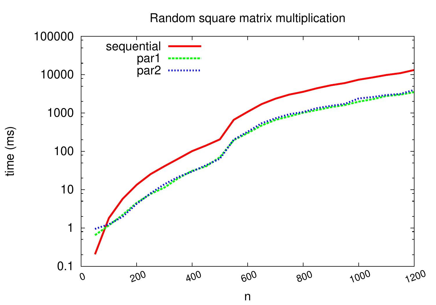
Potential reasons for not obtaining the full linear speedup of \( 4.0 \) are:
Creating and scheduling parallel tasks takes time.
Running the tasks may take different time and the scheduler may not be able to fully use all the threads all the time.
Some other processes were running in the machine so that not all the cores were available all the time.
Transposition
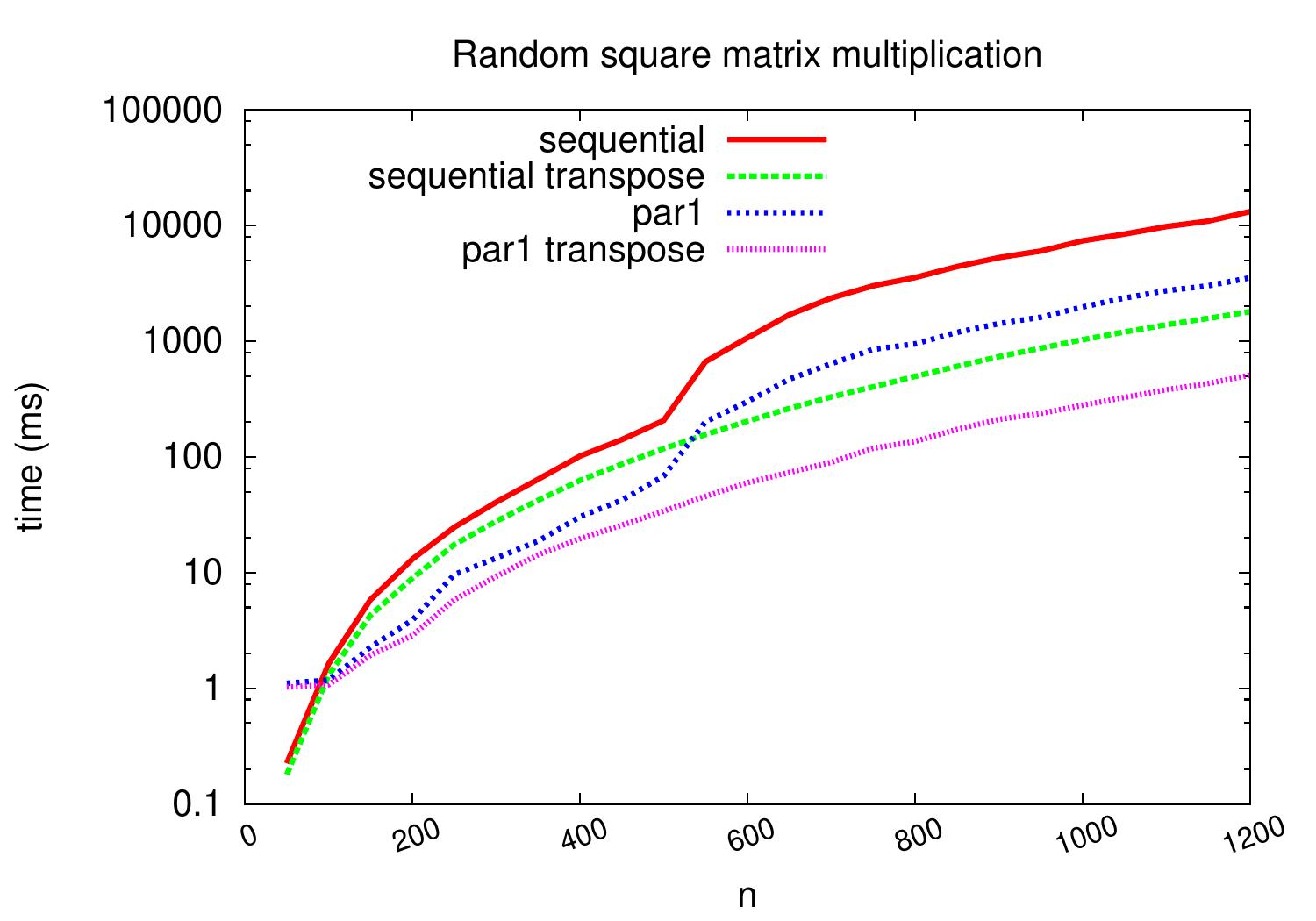
As you may recall, transposing the argument matrix \( B \) before the multiplication did improve the performance of the sequential version. This was because the CPU reads memory not in individual bytes or integers but in larger consecutive memory unit chunks called cache lines (in the case of current Intel processors, cache lines are 64 bytes, which equals to 8 double precision floating point numbers, for instance). In our first sequential and parallel versions, when computing the value \( c_{i,j} \), the consecutive sum terms \( a_{i,k} b_{k,j} \) and \( a_{i,k+1} b_{k+1,j} \) read the values \( b_{k,j} \) and \( b_{k+1,j} \) that are not in consecutive indices but in the indices \( kn + j \) and \( (k+1)n+j \), respectively, when the matrix is stored in the row-major order. Transposing the matrix \( B \) transforms the presentation into column-major order so that the values \( b_{k,j} \) and \( b_{k+1,j} \) are in consecutive indices \( jn + k \) and \( jn + k + 1 \), respectively. We can use this transposition trick in the parallel versions as well.
class Matrix(val n: Int) {
  // LINES REMOVED

  def transpose: Matrix = {
    val r = new Matrix(n)
    for (row <- 0 until n; column <- 0 until n)
        r(column, row) = this(row, column)
    r
  }

  protected def multEntryTranspose(a: Matrix, b: Matrix, row: Int, column: Int): Double = {
    var v: Double = 0.0
    var i = 0
    while(i < a.n) {
      v += a(row, i) * b(column, i)
      i += 1
    }
    v
  }

  def multSeqTranspose(that: Matrix): Matrix = {
    require(n == that.n)
    val that_tp = that.transpose
    val result = new Matrix(n)
    for (row <- 0 until n; column <- 0 until n)
      result(row, column) = multEntryTranspose(this, that_tp, row, column)
    result
  }

  def multPar1Transpose(that: Matrix): Matrix = {
    val that_tp = that.transpose
    val result = new Matrix(n)
    (0 until n).par.foreach(row => {
      for(column <- 0 until n)
        result(row, column) = multEntryTranspose(this, that_tp, row, column)
    })
    result
  }
}
The plot below shows that substantial performance improvements result especially for larger matrices.
Instruction-level parallelism
It is also possible to use parallelism inside a single core.
Modern processors can have several instructions in execution at the same time,
especially if the instructions are independent.
In our previous inner loop we compute the sum by
v = v + a(row, k)*b(column,k) instructions,
increasing the index k in between.
The consecutive v = v + a(row, k)*b(column,k)
and
v = v + a(row, k+1)*b(column,k+1) instructions
are not independent as the second one reads the value of v written by the first.
Thus the second addition cannot be started before the first one has completed.
With partial unrolling of the inner loop and by computing the sum in parts,
we can increase the amount of independence in the inner loops as follows.
class Matrix(val n: Int) {
  // LINES REMOVED

  protected def multEntryTransposeIL(a: Matrix, b: Matrix, row: Int, column: Int): Double = {
    var v1: Double = 0.0
    var v2: Double = 0.0
    var v3: Double = 0.0
    var v4: Double = 0.0
    var i = 0
    val end = a.n & ~0x03
    while(i < end) {
      v1 += a(row, i) * b(column, i)
      v2 += a(row, i+1) * b(column, i+1)
      v3 += a(row, i+2) * b(column, i+2)
      v4 += a(row, i+3) * b(column, i+3)
      i += 4
    }
    var v: Double = v1+v2+v3+v4
    while(i < a.n) {
      v += a(row, i) * b(column, i)
      i += 1
    }
    v
  }

  def multSeqTransposeIL(that: Matrix): Matrix = {
    require(n == that.n)
    val that_tp = that.transpose
    val result = new Matrix(n)
    for (row <- 0 until n; column <- 0 until n)
      result(row, column) = multEntryTransposeIL(this, that_tp, row, column)
    result
  }

  def multPar1TransposeIL(that: Matrix): Matrix = {
    val that_tp = that.transpose
    val result = new Matrix(n)
    (0 until n).par.foreach(row => {
      for(column <- 0 until n)
        result(row, column) = multEntryTransposeIL(this, that_tp, row, column)
    })
    result
  }
}
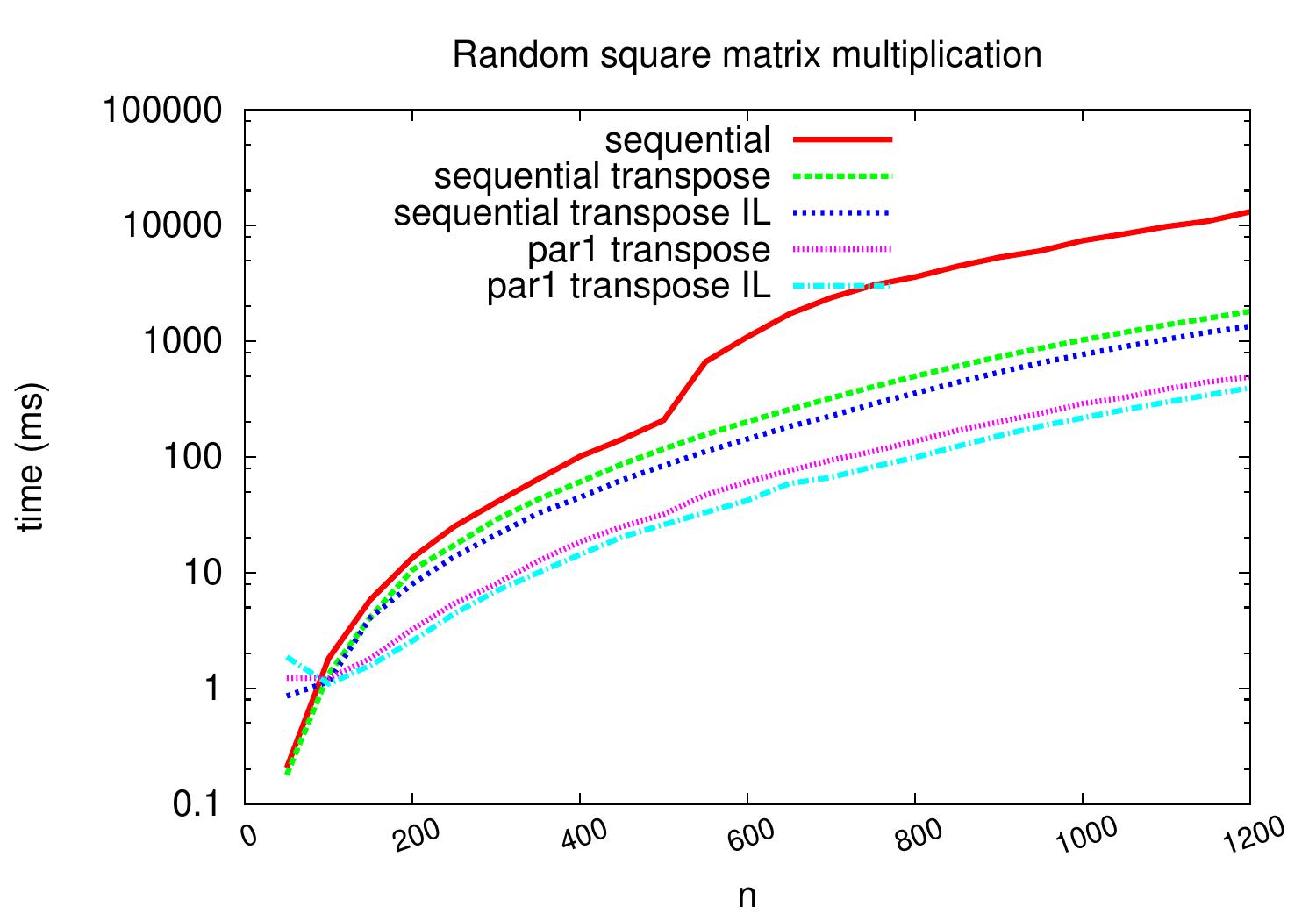
The experimental evaluation results below show that in this case, we are able to get around 20% reduction in running time by this technique.
Modern CPU cores also have vector extensions that allow one to compute an operation on multiple data entries in one instruction. Using these from Scala is not easy and is left out here — see the matrix multiplication code used in the first round lecture of CS-A1120 Programming 2 for how to call C++ programs from Scala/Java and for how to use parallelization and vector extensions in the assembly level in C++.
More on instruction level parallelism (among other things) in the Aalto course CS-E4580 Programming Parallel Computers.