Image filtering with convolution¶

In image processing, one can filter an image by applying a kernel, also called a mask, to it with convolution. Formally, a kernel $ K $ is a $ k \times l $ real matrix (where $ k,l > 0 $ are odd). Applying the kernel to an $ n \times m $ image $ G $ results in the image $ H $ defined as follows $$H(x,y) = \sum_{i=1}^k\sum_{j=1}^l K(i,j) G(x-\Floor{k/2}+i,y-\Floor{l / 2}+j)$$ for all $ \Floor{k/2} \le x < n-\Floor{k/2} $ and $ \Floor{l/2} \le y < m-\Floor{l/2} $. That is, the filtered value of each pixel is the weighted sum of its neighbors. The borders are handled in some manner, for instance, set to zero.

For instance, when we apply the $ 7 \times 7 $ Gaussian blur kernel (with the standard deviation $ \sigma=2.0 $) $$K \approx \left(\begin{smallmatrix}0.005&0.009&0.013&0.015&0.013&0.009&0.005\\0.009&0.017&0.025&0.028&0.025&0.017&0.009\\0.013&0.025&0.036&0.041&0.036&0.025&0.013\\0.015&0.028&0.041&0.047&0.041&0.028&0.015\\0.013&0.025&0.036&0.041&0.036&0.025&0.013\\0.009&0.017&0.025&0.028&0.025&0.017&0.009\\0.005&0.009&0.013&0.015&0.013&0.009&0.005\end{smallmatrix}\right)$$ 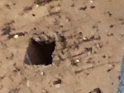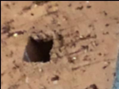to the image on the left below, the result is the image on the right (only the upper left corner of the $ 4032 \times 3024 $ image is shown).

Example: Gaussian blur filtering with a 7×7 kernel (σ = 2.0)¶
Original¶	Filtered¶

The straightforward sequential implementation of the approach has the running time (work and span) of $ \Oh{nmkl} $ because $ \Oh{kl} $ operations are needed to compute the value of each $ n m $ pixels (assuming that $ k $ and $ l $ are small compared to $ n $ and $ m $).

Applying a kernel to an image is an embarrassingly parallel problem as the value $$H(x,y) = \sum_{i=1}^k\sum_{j=1}^l K(i,j) G(x-\Floor{k/2}+i,y-\Floor{l / 2}+j)$$ of each result image pixel can be computed independently and thus concurrently. A parallel version that computes the value of each result pixel in parallel will have the following characteristics:

Work is $ \Oh{nmkl} $ because $ \Oh{kl} $ operations are needed to compute the value of each $ n m $ pixels.
Span is $ \Oh{kl} $ as this is the running time of computing the value of a single output pixel and the pixels are computed in parallel in the ideal case.
The amount of parallelism is thus $ \Oh{nm} $.

Let’s now compare the performance of a straightforward Scala implementation of the sequential version against the parallel version that uses a parallel for-loop to parallelize the individual pixel computations. Running times for a Gaussian $ 7 \times 7 $ kernel on a $ 4032 \times 3024 $ image, with a quad-core desktop machine, are as follows:

Sequential: 26.72s
Parallel: 7.01s
Speedup = 3.8

Of course, easy parallelization is no excuse for not trying to improve an algorithm. In the case of applying Gaussian blur kernel to images, further speedup can be obtained by noticing that Gaussian blur is a separable filter. For instance, the $ 7 \times 7 $ kernel $$\left(\begin{smallmatrix}0.005&0.009&0.013&0.015&0.013&0.009&0.005\\0.009&0.017&0.025&0.028&0.025&0.017&0.009\\0.013&0.025&0.036&0.041&0.036&0.025&0.013\\0.015&0.028&0.041&0.047&0.041&0.028&0.015\\0.013&0.025&0.036&0.041&0.036&0.025&0.013\\0.009&0.017&0.025&0.028&0.025&0.017&0.009\\0.005&0.009&0.013&0.015&0.013&0.009&0.005\end{smallmatrix}\right) \approx v^T v$$ where $ v \approx \left(\begin{smallmatrix}0.070&0.131&0.191&0.216&0.191&0.131&0.070\end{smallmatrix}\right) $. In general, for separable $ k \times l $ filters, one can

apply an $ 1 \times l $ kernel to the original image, and then
apply a $ k \times 1 $ kernel to the intermediate result.

That is, one first performs filtering horizontally on individual rows and then filtering vertically on individual columns (or vice versa). The sequential version has the work and span $ \Oh{nmk+nml} $. Again, both phases can be parallelized, resulting in an algorithm having the work $ \Oh{nmk+nml} $, span $ \Oh{k+l} $, and the amount of parallelism $ \Oh{nm} $.

The running times for applying a Gaussian $ 7 \times 7 $ kernel on a $ 4032 \times 3024 $ image, with a quad-core machine, are now as follows:

Performance of a simple Scala implementation: applying a 7×7 Gaussian blur kernel on a 4032×3024 image in a quad-core machine¶
Sequential	Sequential separable	Parallel	Parallel separable
26.72s	4.30s	7.01s	1.50s
26.72s	4.30s	7.01s	1.50s