Example: Implementing parallel count
As a simple example of using the Fork-join framework,
let’s implement a parallel version of the count method found in Scala collections.
It applies the argument predicate pred to
all the elements in an array a and
returns the number of elements that satisfy the predicate.
That is, we want to build a parallel algorithm that computes the same as
the standard Scala library method application
a.count(pred).
Observe that in the scala.collection.parallel.mutable library of Scala 2.12,
this kind of parallel version is already implemented and
one can use it with a.par.count(pred).
But let’s build our own with the fork-join framework and
see how it compares to the standard library implementation.
Our sequential reference version used in the benchmarks,
call it the “while-loops” version in the sequel,
is as follows:
def count[A](a: Array[A], pred: A => Boolean): Int = {
  var count = 0
  var i = 0
  while(i < a.length) {
    if(pred(a(i))) count += 1
    i += 1
  }
  count
}
Assuming that each predicate evaluation takes constant time, the running time of the sequential version is \( \Theta(n) \).
A non-recursive parallel version
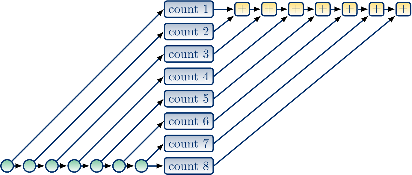
In our first parallel version, we simply
divide the array of \( n \) elements into \( k \) roughly equal-sized chunks,
compute, in parallel, the number of elements satisfying the predicate in each chunk, and
return the sum of these sub-results.
Let’s study the work and span of this parallel version.
If the chunk size is roughly \( d \) for some constant \( d \), then there are \( k \approx \frac{n}{d} \) chunks. Creating the tasks and computing the final sum thus take linear time \( \Theta(n/d) = \Theta(n) \). Evaluating the elements in each chunk in turn takes constant time \( \Theta(d) \). Thus the work is \( \Theta(n/d + d n/d + n / d) = \Theta(n) \) and the span is \( \Theta(n/d + d + n/d) = \Theta(n) \).
As a summary: if one divides the array into too many chunks, then the times needed to launch the tasks and collect the results may start to play a significant role in the running times.
On the other hand, if the number of chunks \( k \) is a constant, then evaluating the predicate in each chunk takes time \( \Theta(\frac{n}{k}) \). The work is now \( \Theta(k + k \frac{n}{k} + k) = \Theta(n) \) while the span is \( \Theta(k + \frac{n}{k} + k) = \Theta(n) \).
Thus in theory the algorithm is not very attractive as the span is linear in both cases. However, this simple version may work well in practice currently as the number of available cores is small compared to the typically large arrays we wish to handle. Suppose that we have \( P \) computing cores in use. What is a good value for \( k \), i.e., how many chunks should we take?
If we take \( k = n \), then we get maximum parallelism available from our \( P \) threads but launching the tasks and job scheduling probably becomes too costly when \( n \) is large.
If we take \( k = P \) and the computing time of the predicate is not always the same, then there is a risk that some tasks take much longer time than some others and we do not get maximum parallelism as some cores are idle while some are still working.
Maybe a good compromise is to take \( k = 16 P \) (or \( n \) if \( n < 16 P \)) so that there are enough but not too many tasks.
The algorithm is easy to implement with our par.task construction.
def countPar[A](a: Array[A], pred: A => Boolean): Int = {
  val N = a.length
  val P: Int = par.getParallelism
  val nofTasks = N min P * 16
  val starts = (0 to nofTasks).map(i => (N * i) / nofTasks)
  val intervals = (starts zip starts.tail)
  // Start the parallel tasks
  val countTasks = intervals.map({
    case (start, end) => par.task {
      var i = start
      var count = 0  // A private variable for the sub-result
      while(i < end) {
	if(pred(a(i)))
	  count += 1
	i += 1
      }
      count  // Return the sub-result
    }
  })
  // Wait until all tasks have finished, get the sub-results
  val counts = countTasks.map(_.join())
  // Return the sum of the sub-results
  counts.sum
}
Incorrect: data races
To illustrate a typical mistake made in implementing concurrent programs,
consider the incorrect Scala program variant below.
As the result variable is shared between the concurrent tasks,
it contains a data race
and
will most likely give an incorrect result.
def countParBad[A](a: Array[A], pred: A => Boolean): Int = {
  val N = a.length
  val P: Int = par.getParallelism
  val nofTasks = N min P * 16
  val starts = (0 to nofTasks).map(i => (N * i) / nofTasks)
  val intervals = (starts zip starts.tail)
  var result = 0  // BAD: a non-atomic variable shared by tasks
  val countTasks = intervals.map({
    case (start, end) => par.task {
      var i = start
      while(i < end) {
	if(pred(a(i)))
	  result += 1  // BAD: a non-atomic update
	i += 1
      }
    }
  })
  // Wait until all tasks have finished
  countTasks.foreach(_.join())
  result // Return the most-likely-INCORRECT result
}
Potentially inefficient: atomic updates
In this example, the data race problem discussed above could be fixed by using atomic variable updates (see, for instance, Atomic Variables in the Java Tutorials or the atomic class in the C++ standard library).
def countParAtomic[A](a: Array[A], pred: A => Boolean): Int = {
  val N = a.length
  val P: Int = par.getParallelism
  val nofTasks = N min P * 16
  val starts = (0 to nofTasks).map(i => (N * i) / nofTasks)
  val intervals = (starts zip starts.tail)
  val result = new java.util.concurrent.atomic.AtomicInteger()
  val countTasks = intervals.map({
    case (start, end) => par.task {
      var i = start
      while(i < end) {
	if(pred(a(i))) result.addAndGet(1) // Atomically increment result by one
	i += 1
      }
    }
  })
  // Wait until all tasks have finished
  countTasks.foreach(_.join())
  result.get()
}
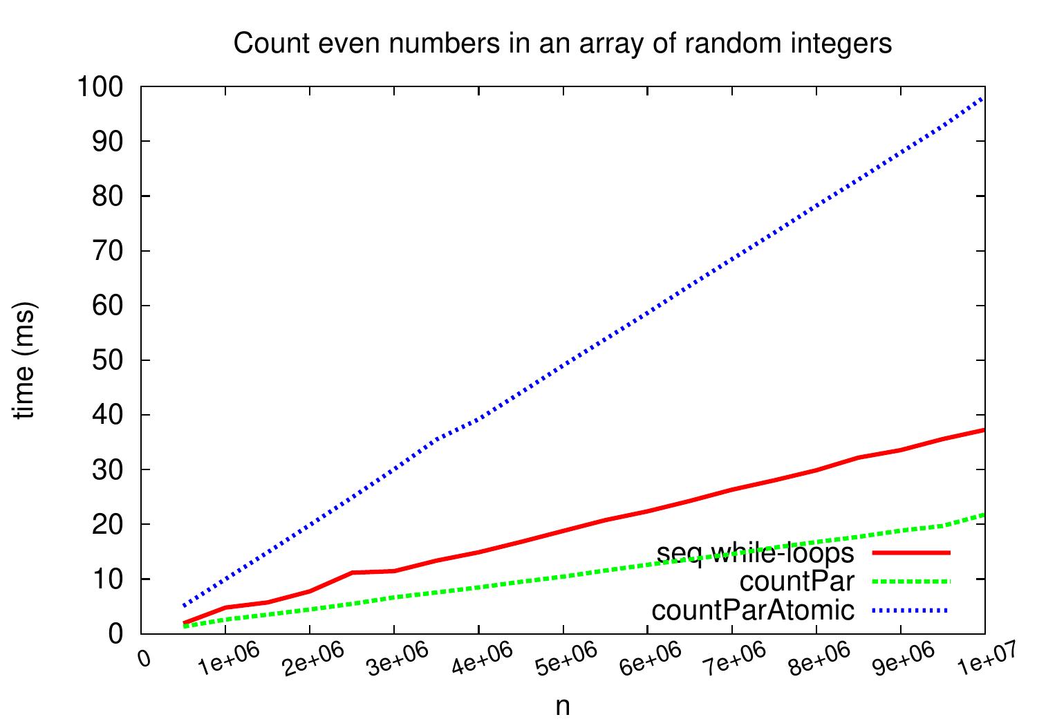
However, the atomic updates require some synchronization and thus can incur a considerable performance penalty if the atomic updates are done very often. As an example, the plot below compares the performance of this atomic update version to that of the sequential and parallel versions above on inputs that cause very frequent atomic updates. The difference would not be that radical on inputs where the predicate evaluation takes more time and fewer of the input elements actually fulfill the predicate, though.
Potentially inefficient: false sharing
To illustrate a second potential source of inefficiency
called false sharing,
consider the Scala version below.
The code does not have data races as the sums are computed in different elements
in the results array.
However,
parallel tasks may write to neighboring indices of the results array.
This may cause nonoptimal performance for the following reason.
When a core reads a value from the memory,
the value is read to a cache memory
that is faster and closer to the core than the main memory.
The cache entries, called cache lines,
do not cache individual bytes or words of the main memory but larger chunks.
For instance, in the current Intel processors,
the size of a cache line is 64 bytes, which equals to 16 32-bit integers, for instance.
If different cores write to the same cache line,
a cache coherence protocol has to maintain their consistency and
this causes extra communication between the cores.
In our example, different tasks may write to the same cache line if they write to
neighboring indices of the results array.
def countParFalseSharing[A](a: Array[A], pred: A => Boolean): Int = {
  val N = a.length
  val P: Int = par.getParallelism
  val nofTasks = N min P * 16
  val starts = (0 to nofTasks).map(i => (N * i) / nofTasks)
  val intervals = (starts zip starts.tail);
  val results = Array.ofDim[Int](nofTasks)  // Results of the tasks
  val countTasks = intervals.zipWithIndex.map({
    case ((start, end), index) => par.task {
      var i = start
      while(i < end) {
	if(pred(a(i)))
	  results(index) += 1 // No data race but may write to the same cache line
	i += 1
      }
    }
    })
  // Wait until all tasks have finished
  countTasks.foreach(_.join())
  // Return the sum of the subresults
  results.sum
}
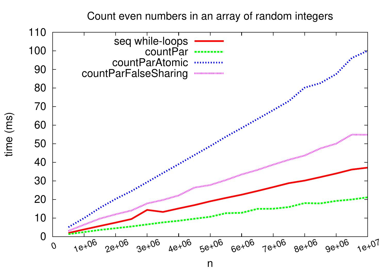
The plot below shows that false sharing can cause significant performance penalty
if writes to the same cache line are very frequent.
Again,
the performance penalty would not be that large on inputs that cause less
frequent writes to the results array (predicate evaluation takes more time or less elements satisfy the predicate).
Our first parallel version did not have this false sharing problem
because each sub-sum is computed in a private variable count,
which is stored in a register or in the stack memory of the executing thread.
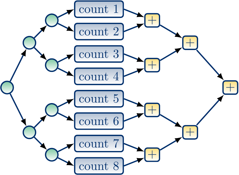
A recursive version
We can also make a recursive version. It follows the divide-and-conquer paradigm:
If the array is small enough, compute the result sequentially.
Otherwise, split the array in two equally-size sub-arrays.
Then, recursively and in parallel, compute the results for the two sub-arrays.
Finally, return the sum of the two sub-array results.
In this recursive version, the creation of new tasks as well as the final sum computation are also parallelized. If we split the array until there is only one element left, the worst-case span can be obtained from the recurrence $$T(1) = c \text{ and } T(n) = d+ \max\Set{T(\Floor{n/2}),T(\Ceil{n/2})}$$ where \( c \) is the time taken for the predicate computation and \( d \) is some constant. Substituting \( n = 2^k \) for some non-negative \( k \), we get \( T(2^k) = d + T(2^{k-1}) = … = kd + c \). Thus the worst-case span is \( T(n) = c + d\Lg{n} = \Theta(c + \Lg{n}) \). If the predicate can be evaluated in constant time, it is possible to count the number of elements satisfying the predicate in logarithmic time when \( \Theta(n) \) computing resource are available.
The work is also \( \Theta(n+cn)=\Theta(cn) \) because the recursive divisions and the final sum computation are done with \( \Theta(n) \) steps.
We can implement the recursive version with
the par.parallel methods instead of par.task.
In practice, we do not perform full recursion but
stop when “small enough” sub-arrays are considered.
Thus we have to decide how large is a “small enough” sub-array:
It cannot be \( 1 \) on large arrays as then the parallel forks take too much time
Neither should it be \( n / P \) if the predicate computing times can vary
Let’s use \( n / (16 P) \) as a compromise
def countParRec[A](a: Array[A], pred: A => Boolean): Int = {
  val P: Int = par.getParallelism
  val smallArrayThreshold: Int = 1 max a.length / (P * 16)
  def inner(start: Int, end: Int): Int = {
    if(end - start <= smallArrayThreshold) {
      // Small sub-arrays are handled sequentially
      var count = 0
      var i = start
      while(i <= end) {
	if(pred(a(i))) count += 1
	i += 1
      }
      count
    } else {
      // Longer sub-arrays are split and handled (recursively) in parallel
      val mid = start + (end - start) / 2
      val (countLeft, countRight) = par.parallel(
	inner(start, mid),
	inner(mid+1, end)
      )
      // Return the sum of the sub-array results
      countLeft + countRight
    }
  }
  inner(0, a.length-1)
}
Experimental evaluation
Let’s benchmark the Scala codes given above against themselves and
the methods Array.count(pred) and Array.par.count(pred)
in the Scala library.
Again, we use a Linux Ubuntu machine with Intel Xeon E31230 quad-core CPU running at 3.2GHz and report wall clock times.
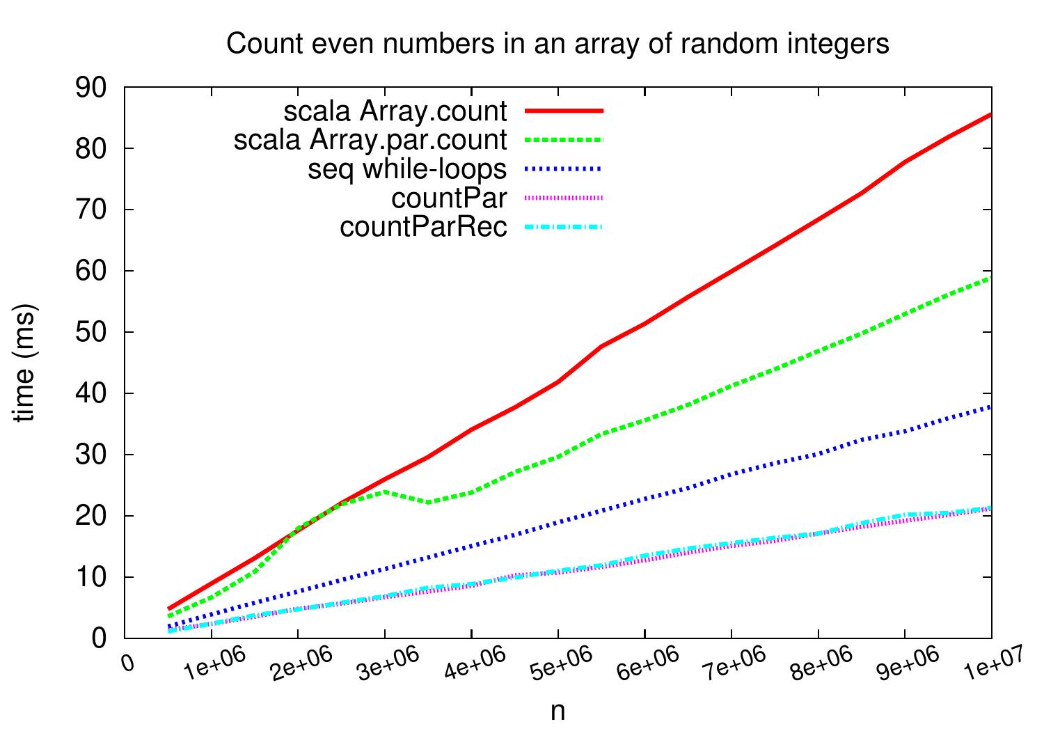
In the first benchmark family,
we count the number of even integers in random integer arrays.
As can be seen in the plot below,
we obtain a speedup of \( \approx 1.7 \) when compared to the sequential “while-loop” version on large arrays.
In this case, the predicate evaluation is very fast and
the task creation, scheduling and joining times can play a role in that the speedup is
not close to four.
Our non-recursive and recursive parallel versions perform very similarly as expected:
at the end, they split the array in roughly same number of equally-sized chunks
and
parallelizing the task creation phase does not help too much when the number of available cores (and thus the number of chunks) is relatively small.
On this kind of benchmark, the count method of Scala collections
performs slightly worse,
probably because its code is build by using generic templates to avoid code duplication.
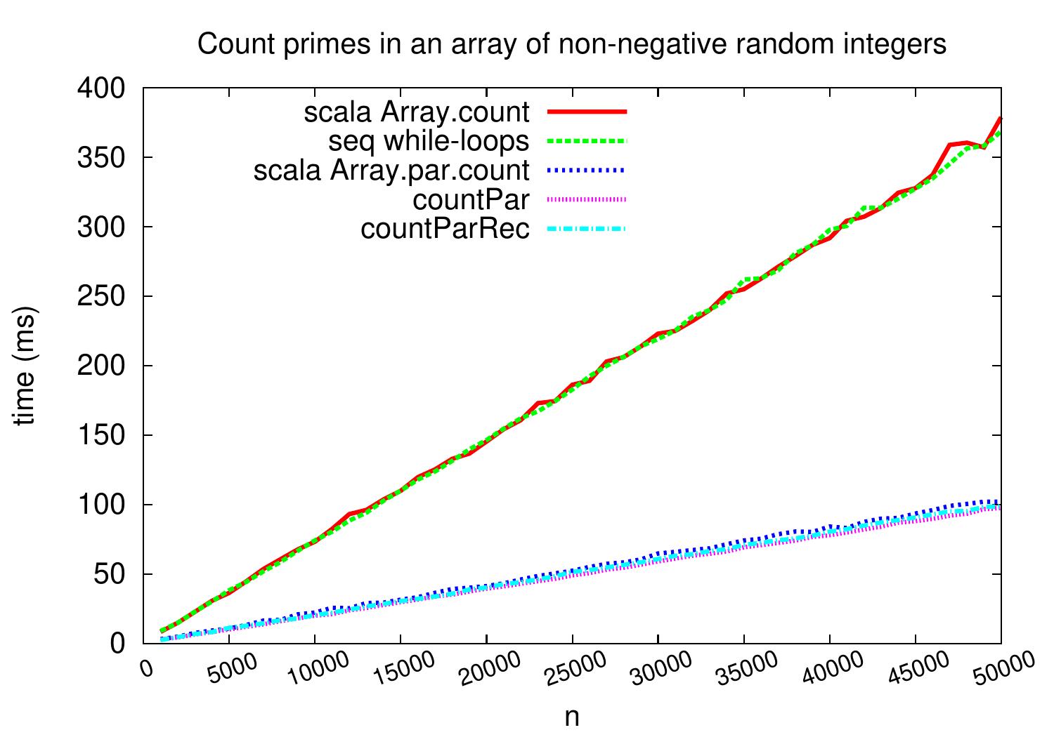
As a second benchmark family, let’s see what happens if we count the amount of prime numbers in an array of non-negative random numbers. The applied non-primality test is the straightforward one checking whether there is an integer \( i \in [0 .. \lceil\sqrt{x}\rceil] \) dividing \( x \). The results below show a speedup of almost 4 with all the parallel versions. The explanation is that here the time is spent mostly in the primality tests and the task creation times etc do not play that significant role.