Threads¶

(The following is partly recap from CS-A1120 Programming 2)

Threads are the core mechanism of executing code concurrently in multicore machines. Threads execute

in parallel in different cores when available, or
in time slices when there are not enough cores for all the active threads.

Different threads within the same process, such as a Scala application or a C++ program, share memory and can thus access same data structures. Each process has at least one thread, the main thread. As Scala programs run on top of a Java virtual machine, they use Java threads. To perform computations concurrently,

threads can start new threads (“fork”),
wait until other threads have finished (“join”), and
communicate between each other through the shared memory.

Communication between threads is a source of many errors and if done, one should take care of proper synchronization or use high-level concurrency objects. Please observe that debugging errors in concurrent programs can be much more difficult than in sequential programs because the timing of the thread executions cannot usually be controlled: a bug can appear in one execution but not in the next one because the threads are executed in a slightly different schedule. As stated earlier, in this course we will not discuss thread communication and synchronization further but assume that the tasks executed in threads are independent and the only synchronization is at the end when the threads join.

Example

Computing the median and average of an array in parallel by using Java threads in Scala can be done as follows.

abstract class ArrayRunnable[T](val a: Array[T]) extends Runnable {
  var result: Int = 0
}
val medianRunnable = new ArrayRunnable(a) {
  def run() = {result = a.sorted.apply(a.length / 2)}
}
val avgRunnable = new ArrayRunnable(a) {
  def run() = {result = a.sum / a.length}
}
val medianThread = new Thread(medianRunnable)
val avgThread = new Thread(avgRunnable)
// Run the threads in parallel
medianThread.start()
avgThread.start()
// Synchronize: wait until both have finished
medianThread.join()
avgThread.join()
// Get the results: joins quarantee that they are ready
val (median, avg) = (medianRunnable.result, avgRunnable.result)

Assume that threads are only created with forks and then later joined but no other synchronization is done. In such a case, each execution can be illustrated with a computation DAG in which vertices correspond to different points of execution in each thread: entry, fork, join, and exit. Consecutive execution points in a thread are connected with edge

Each fork vertex is connected to the entry vertex of the created thread.
Each exit vertex in a non-main thread is connected to the corresponding join vertex.

Example

The computation DAG for an execution where the main thread forks two new threads that compute the median and average of an array in parallel:

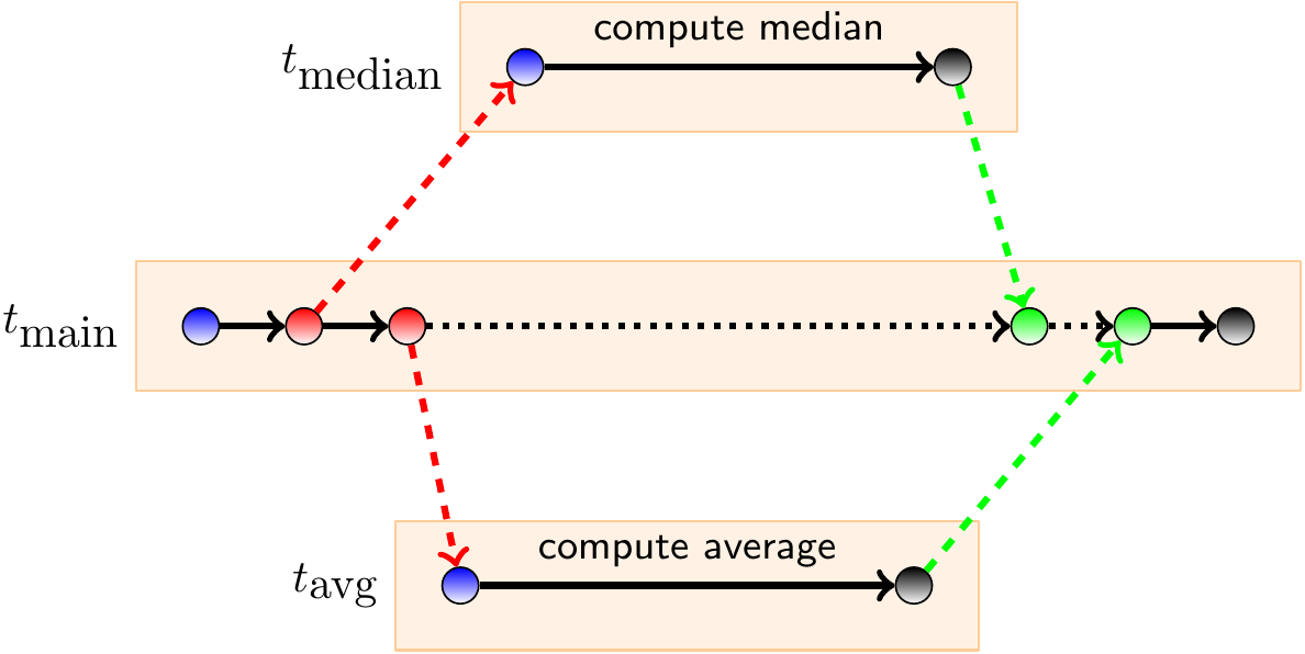
Recall that the work of a parallel program is the sum of execution times of all its parallel computations (\( \approx \) the number of CPU cycles used in all the threads). In the DAG presentation, this is the sum of the running times of all the computation edges.

On the other hand, the span is the “wall clock time” of the program in an ideal setting with unbounded amount of parallel processing units. In the DAG presentation, this corresponds to the length of the longest path.

Example

Recall our previous example of computing the median and average of an array in parallel by using Java threads in Scala:

abstract class ArrayRunnable[T](val a: Array[T]) extends Runnable {
  var result: Int = 0
}
val medianRunnable = new ArrayRunnable(a) {
  def run() = {result = a.sorted.apply(a.length / 2)}
}
val avgRunnable = new ArrayRunnable(a) {
  def run() = {result = a.sum / a.length}
}
val medianThread = new Thread(medianRunnable)
val avgThread = new Thread(avgRunnable)
// Run the threads in parallel
medianThread.start()
avgThread.start()
// Synchronize: wait until both have finished
medianThread.join()
avgThread.join()
// Get the results: joins quarantee that they are ready
val (median, avg) = (medianRunnable.result, avgRunnable.result)

The work is the sum of

the times taken in thread allocations, initialization and deallocation, and
the sum of the times taken in the median and average computations.

The span is the sum of

the times taken in thread allocations, initialization and deallocation, and
the larger of the times taken in the median and average computations.

However, programming with plain threads is tedious and error prone. Furthermore, creating and deleting threads is not cheap:

Thread objects use a significant amount of memory, and in a large-scale application, allocating and deallocating many thread objects creates a significant memory management overhead. (An excerpt from Java tutorials.)

In the rest of the round, we will use higher level abstractions where the thread management is taken care by a concurrency platform and we can focus on tasks that should be run in parallel. The main thing we have to take care is that there are no data races. This is usually quite easy to obtain: just make sure that tasks that can run in parallel will never read values written by the others.