Mergesort
Mergesort is a commonly used, important sorting algorithm. Although it was introduced already in 1945, variants of it are still used nowadays. For instance,
the stable_sort method in the current GNU C++ standard library implementation uses a variant of mergesort,
the java.util.Arrays.sort methods on object arrays use a variant of mergesort, and
the Timsort algorithm used in the current Python implementation is based on mergesort.
For a history of mergesort, see the following article:
Donald E. Knuth: Von Neumann’s First Computer Program. ACM Computing Surveys 2(4):247–260, 1970.
Mergesort has a guaranteed \( \Oh{n \Lg n} \) worst-case running time. The high-level idea is as follows:
If we have two consecutive sorted sub-arrays, it is easy to merge them to a sorted array containing the elements of both sub-arrays.
Therefore, we can
recursively divide the input array into smaller consecutive sub-arrays until they are easy to sort (for instance, until they are of size 1), and
then merge the results into longer and longer sorted sub-arrays until the whole array is sorted.
Mergesort thus follows the divide and conquer algorithm design paradigm. In general, the paradigm has three phases:
Divide: The problem is recursively divided into smaller subproblems until they become easy enough.
Conquer: The small subproblems are solved.
Combine: The results of the subproblems are then combined to give a solution to the original problem.
Example: High-level idea of mergesort
The high-level idea of mergesort can be illustrated with an example array as follows.
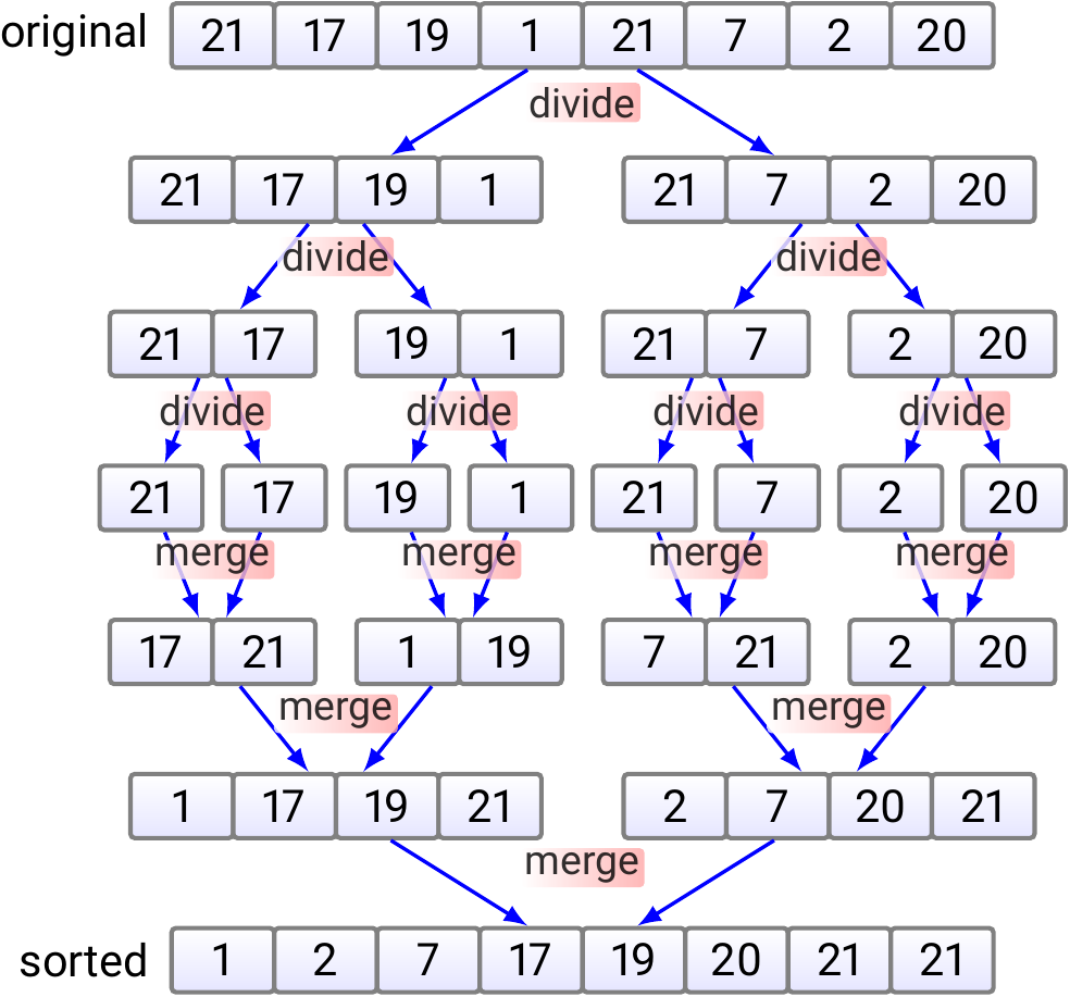
The three divide-and-conquer paradigm phases are:
Divide: First, the original array is divided into smaller sub-arrays. In a real implementation, the subarrays are not explicitly constructed but they are implicitly represented by their start and end indices.
Conquer: When the sub-arrays are of size one, they are each individually sorted. Thus the conquering phase does no real work in this case.
Combine: Finally, the small sorted sub-arrays are merged into larger sorted sub-arrays until the whole array is sorted.
Implementing the merge operation
In the division phase, we split a sub-array into two consecutive sub-arrays. As explained in the example above, there is no need to copy the sub-arrays anywhere but maintaining the start and end indices is enough.
In the merge phase, the sorted sub-arrays to be merged are also consecutive. To make the larger merged sub-array, we first merge the sorted sub-arrays in an auxiliary array and then copy the result back to the original array. To perform the merge of two sub-arrays, we maintain two indices, \( i \) and \( j \), in the smaller sub-arrays. Initially, they are the start indices of the smaller sub-arrays. Then, at each step, we append the smaller value in these indices to the auxiliary array and increase the index in question. This is continued until both sub-arrays have been processed. Finally, we copy the resulting larger sub-array from the auxiliary array back to the original array.
Example: Merging two consecutive, sorted sub-arrays.
Suppose that we have an array \( \Arr{a_0,a_1,…,a_7} \) of eight elements
and
we have already sorted the consecutive sub-arrays
\( \Arr{a_0,a_1} \) and \( \Arr{a_2,a_3} \).
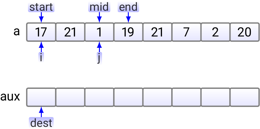
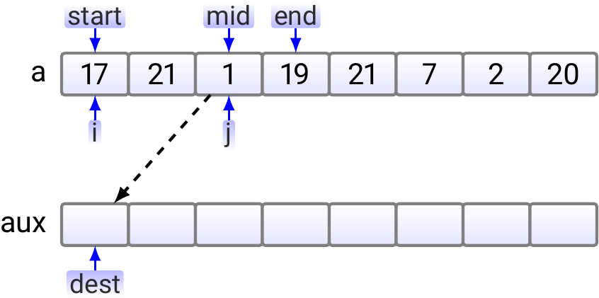
In the merge algorithm,
let start be the start index \( 0 \) of the first sub-array,
mid be the start index \( 2 \) of the second sub-array
(it is the “mid-point” of the resulting larger sub-array \( \Arr{a_0,a_1,a_2,a_3} \)),
and end be the end index \( 3 \) of the second sub-array.
Furthermore, the dest index tells the index in the auxiliary array
in which the next element in the merged sub-array should be inserted.
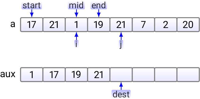
In the beginning, the situation is as shown below.
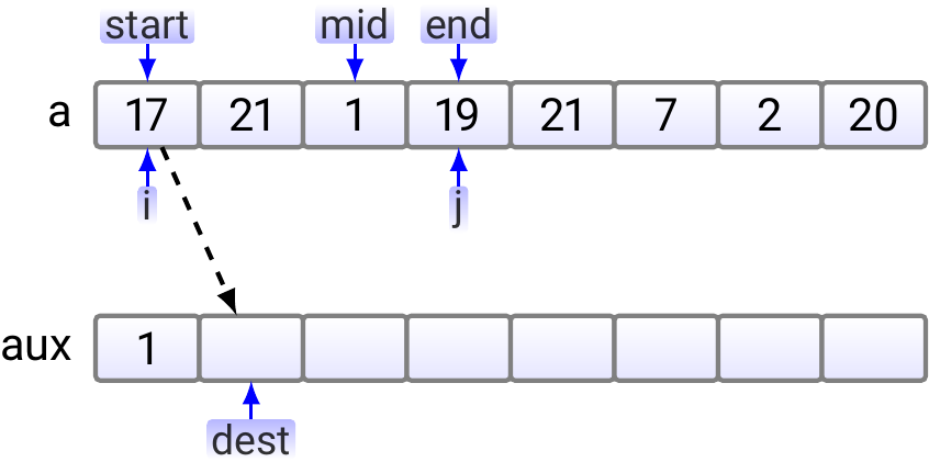
In the first step, we compare 17 and 1; 1 is smaller and thus copied to the auxiliary array.
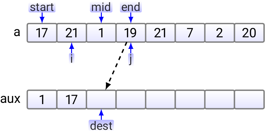
Next, as \( 17 < 19 \), 17 is copied to the aux array.
As \( 19 < 21 \), \( 19 \) is copied to the aux array.
Now the right sub-array index \( j \) is out of the sub-array and we copy the rest of the left sub-array to the auxiliary array.
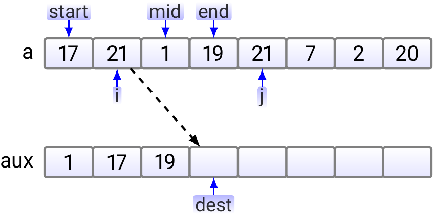
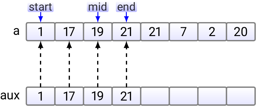
After that, the situation is as shown below.
Finally, we copy the merged sub-array back to the original array.
An implementation of the merge operation in Scala is given below.
def merge(a: Array[Int], aux: Array[Int], start: Int, mid: Int, end: Int): Unit = {
  // Initialize the index variables
  var (i, j, dest) = (start, mid, start)
  // Merge the subarrays to the aux array
  while (i < mid && j <= end) {
    if (a(i) <= a(j)) { aux(dest) = a(i); i += 1 }
    else { aux(dest) = a(j); j += 1 }
    dest += 1
  }
  while (i < mid) { aux(dest) = a(i); i += 1; dest += 1 }  // Copy rest
  while (j <= end) { aux(dest) = a(j); j += 1; dest += 1 } // Copy rest
  // Copy back from aux to a
  dest = start
  while (dest <= end) { a(dest) = aux(dest); dest += 1 }
}
It is easy to see that the running time of the merge operation is \( \Theta(k) \), where \( k \) is the sum of the sizes of the two consecutive sub-arrays.
The main routine
Once we have the merge routine, the recursive mergesort algorithm itself is rather simple and elegant:
def mergesort(a: Array[Int]): Unit = {
  if (a.length <= 1) return

  // Auxiliary memory for doing the merges
  val aux = new Array[Int](a.length)

  // The recursive main algorithm
  def _mergesort(start: Int, end: Int): Unit = {
    if (start >= end)
      return // One or zero elements, do nothing
    val leftEnd = start + (end - start) / 2   // The midpoint
    _mergesort(start, leftEnd)        // Sort the left half
    _mergesort(leftEnd + 1, end)      // Sort the right half
    merge(a, aux, start, leftEnd + 1, end)  // Merge the results
  }
  _mergesort(0, a.length - 1)
}
The code above is for integers arrays, modifying to other element types as well as extending to the generic Ordered trait is again straightforward.
With the above implementations of the merge operation and the main routine, the resulting mergesort implementation is a stable sorting algorithm. An exercise: argument why this is the case.
Running time and memory requirement analysis
A recurrence for the running time of mergesort is $$T(n) = T(\Floor{n/2}) + T(\Ceil{n/2}) + cn$$ and \( T(1) = c£ \), where \( c \) is a positive constant. If \( n \) is a power of two, we can substitute the parameter with \( n = 2^k \) and get $$T(2^k) = T(2^{k-1}) + T(2^{k-1}) + c2^k = c2^k + 2T(2^{k-1})$$ Expanding the recurrence, we obtain \begin{eqnarray*} T(2^k) &=& c2^k + 2(c2^{k-1} + 2T(2^{k-2}))\\ &=& c2^k + 2 c 2^{k-1} + 4(c 2^{k-2} + 2T(2^{k-3}))\\ &=& …\\ &=& (k+1) c 2^k \end{eqnarray*} Recalling that \( k = \Lg{n} \), we get \( T(n) = c n \Lg{n} + cn = \Theta(n \Lg n) \).
We can also analyze the required run-time graphically by showing the computation of \( T(n) \) as a tree:
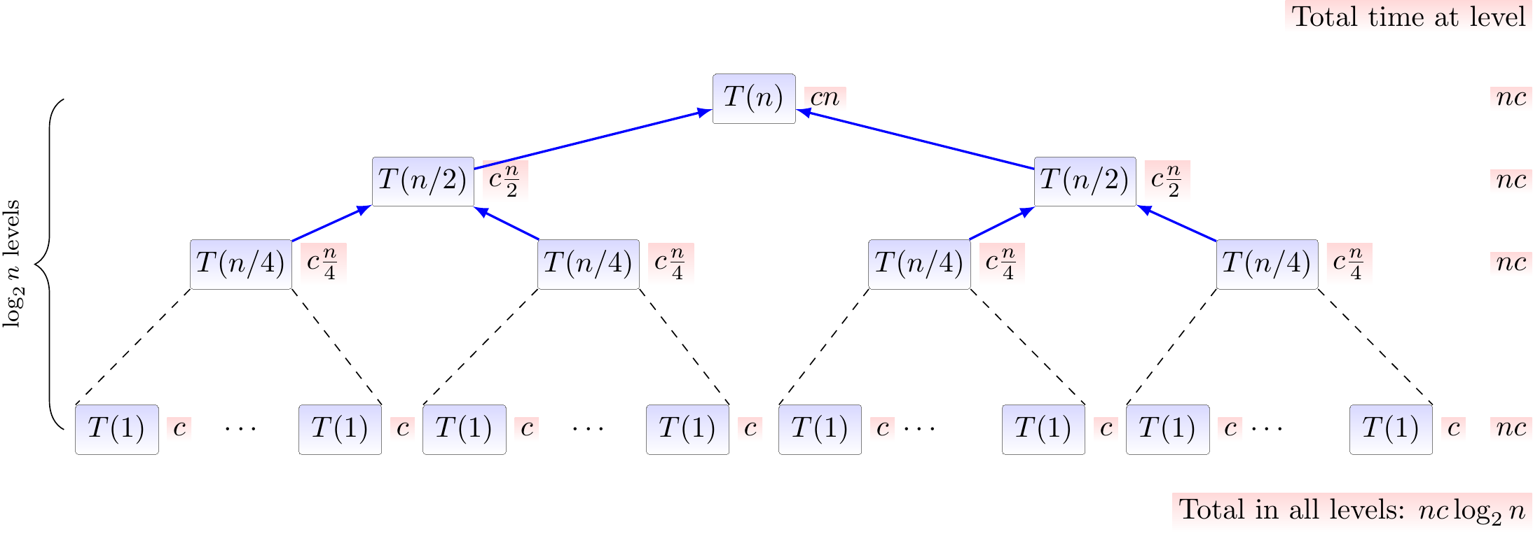
Here we omit the floors and ceilings and use the recurrence $$T(1) = c \text{ and } T(n) = T(n/2) + T(n/2) + cn$$ The red annotations beside nodes illustrate the work done at the node itself. The recursion stops when \( \frac{n}{2^i} \le 1 \), ie. when \( i \ge \Lg n \), and thus the tree has \( \Lg n + 1 \) levels.
Compared to selection and insertion sort algorithms, mergesort uses more memory:
The auxiliary array needed in the merge routine takes \( \Theta(n) \) units of memory.
Furthermore, each stack frame in the recursive calls consumes a constant amount of memory and the maximum recursion depth is \( \Lg{n}+1 \). Thus the recursion needs \( \Oh{\Lg{n}} \) units of extra memory.
As a consequence, mergesort requires \( \Theta(n) \) units of extra memory and does not work in place.
Experimental evaluation
For medium-sized arrays containing random integers, mergesort performs and scales significantly better than insertion sort and scales better as well.
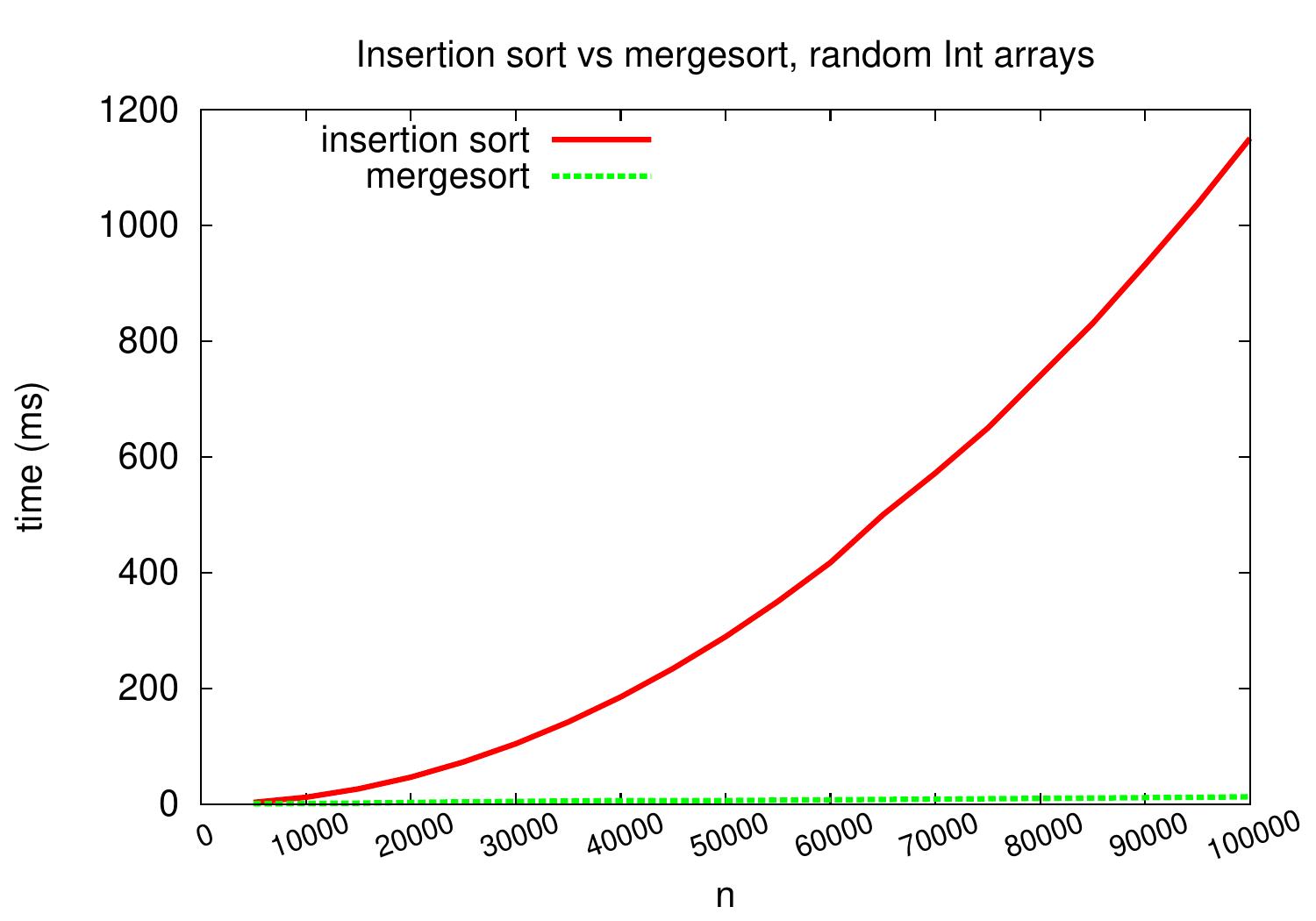
The same plot but with a logarithmic \( y \)-axis scale shows that insertion sort is more than a constant factor slower than mergesort on these kind of input arrays.
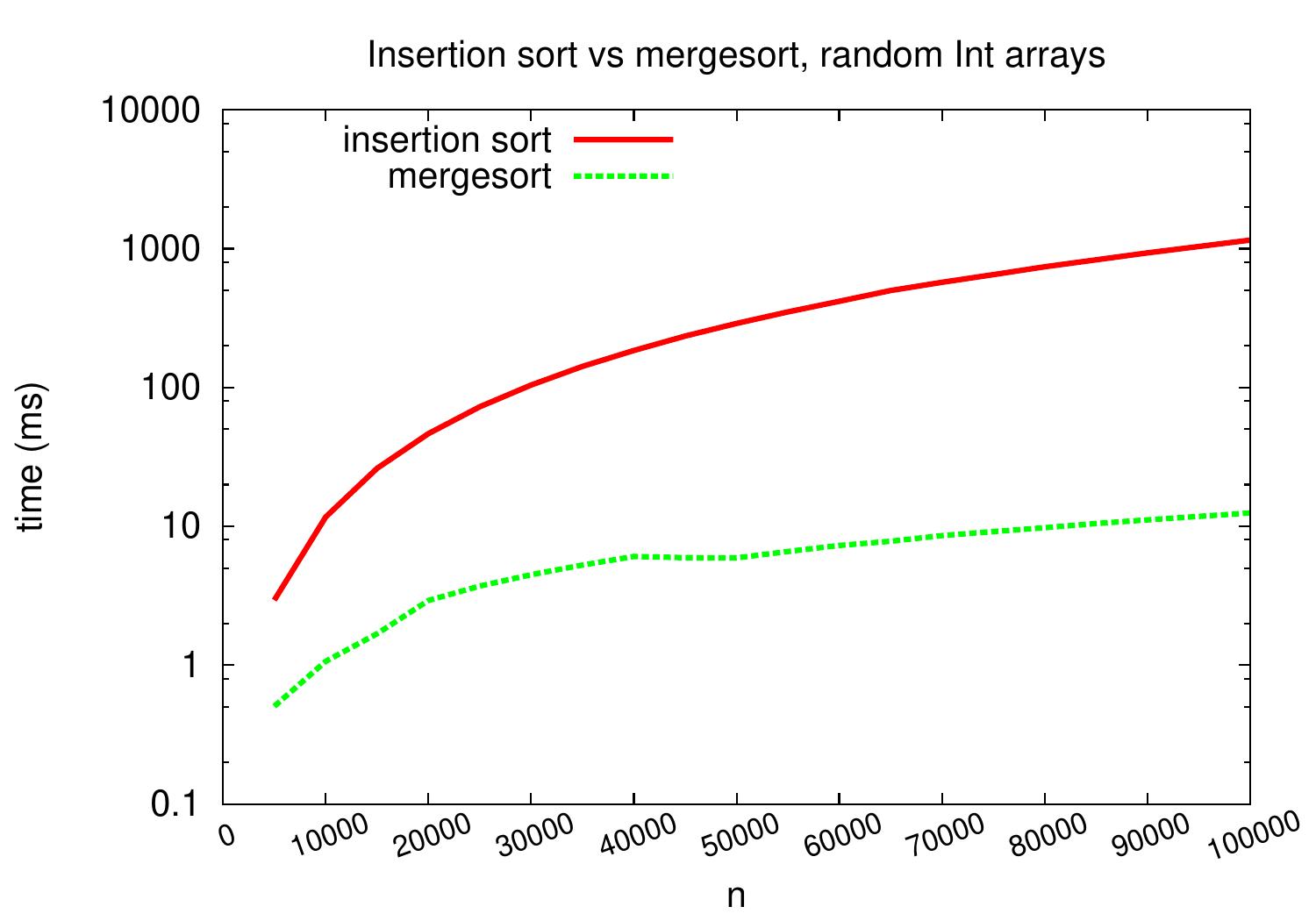
As an example, for arrays with random 100,000 integers, our insertion sort implementation takes over one second but mergesort only takes about 20ms. The exact times depend at least on the applied hardware, Scala compiler and Java VM, but it is clear that mergesort scales much better.
On arrays with random integers, insertion sort is competitive only for very small arrays.
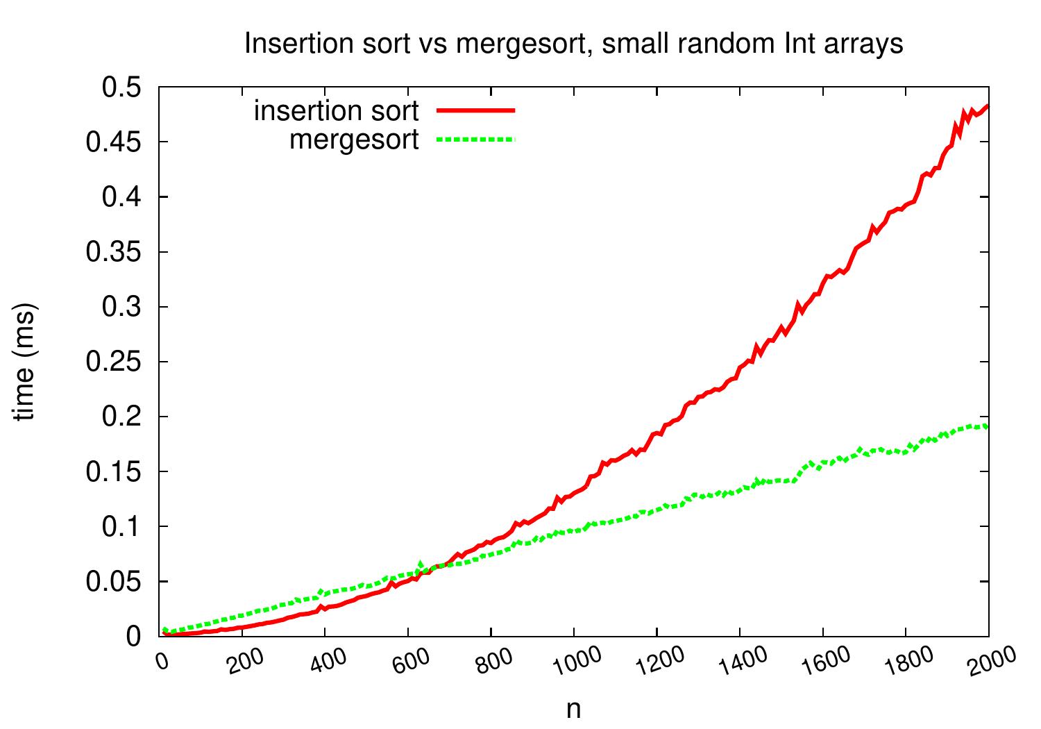
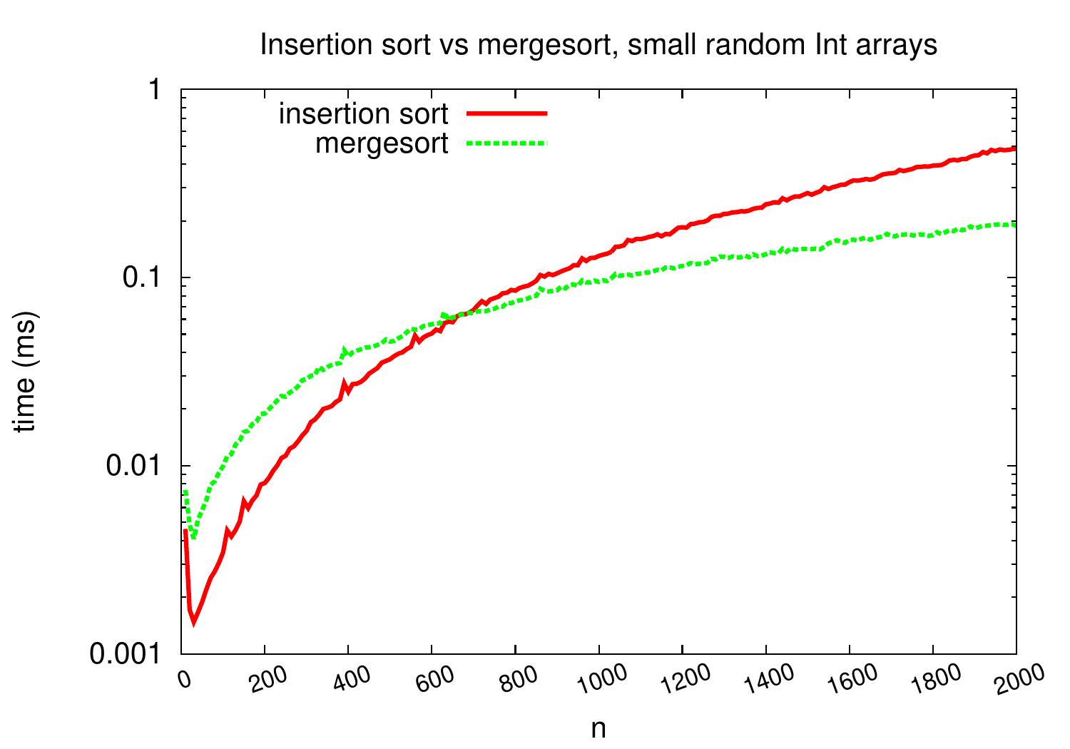
Handling small sub-arrays
In mergesort, each recursive call induces a function invocation and function invocations involve some instructions and memory activity (getting and initializing new stack frame). Observing the relative efficiency of insertion sort on small sub-arrays illustrated in the evaluation above, we may consider an optimized variant of mergesort in which recursion is not performed all the way to unit sized sub-arrays but insertion sort is called for sub-arrays whose size is below some predetermined threshold value. The modification in Scala is quite easy:
def mergesort(a: Array[Int], threshold: Int = 64): Unit = {
  if (a.length <= 1) return
  val aux = new Array[Int](a.length)
  def _mergesort(start: Int, end: Int): Unit = {
    if(end - start < threshold) insertionsort(a, start, end) //Changed
    else {
      val leftEnd = (start + end) / 2
      _mergesort(start, leftEnd)
      _mergesort(leftEnd + 1, end)
      merge(a, aux, start, leftEnd + 1, end)
    }
  }
  _mergesort(0, a.length - 1)
}
Above,
insertionsort(a, start, end) sorts the
subarray a[start..end] with insertion sort.
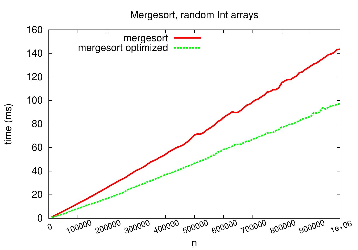
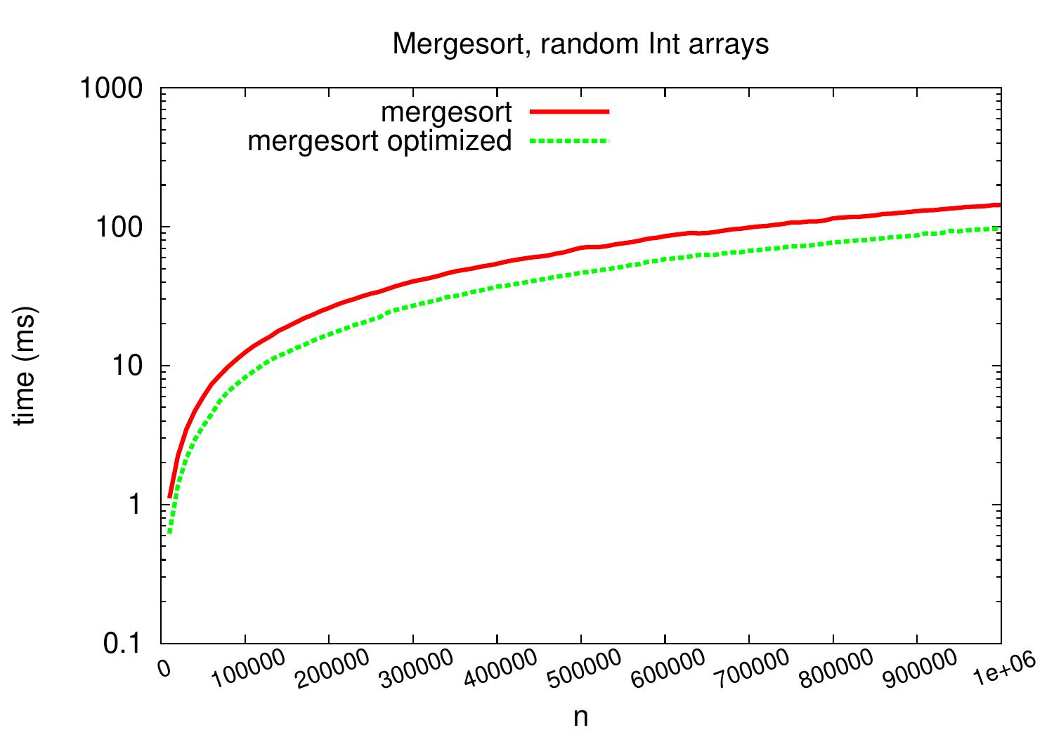
As shown in the experimental results plots below,
a decent constant-factor speedup is achieved: