Selection sort¶

Selection sort is an elementary sorting algorithm based on the following simple idea:

Find a smallest element in the array and swap it with the first one.
Repeat the previous step when considering the sub-array obtained by excluding the first element, until the sub-array consists of only one element.

A straightforward Scala implementation of the algorithm for integer arrays is given below.

def selectionSort(a: Array[Int]): Unit = {
  val n = a.length
  var i = 0 // The first index of the sub-array considered
  while(i < n-1) {
    // Find the smallest element in the sub-array a(i..n-1)
    var smallest_element = a(i)
    var smallest_index = i
    var j = i + 1
    while(j < n) {
      if(a(j) < smallest_element) {
	smallest_element = a(j)
	smallest_index = j
      }
      j += 1
    }
    // Swap the elements at a(i) and a(smallest_index)
    a(smallest_index) = a(i)
    a(i) = smallest_element
    i += 1
  }
}

Example: Selection sort

The animation below shows how selection sort works on a smallish array of integers. Observe how the example illustrates that selection sort is not stable: the relative positions of the elements 10 swap in the sorting process.

Note that only the current minimum element candidate is stored outside the array at any point of time. Thus the amount of extra memory required is \( \Theta(1) \) and the algorithm works in place.

Running time analysis¶

Running time analysis of the algorithm is quite straightforward. The body of the inner while-loop takes constant time. So do all the all instructions, excluding the inner while-loop, in the outer while-loop. For the outer while-loop index \( i \), the inner loop body is executed \( n-1-i \) times. Thus the running time is \( \sum_{i=0}^{n-2}(c + (n-1-i)d) \), where \( c \) and \( d \) are constants capturing the constant running times of the outer while-loop body (excluding the inner while-loop) and the inner while-loop body. The sum expands to \( (n-1)c + d((n-1) + (n-2) + … + 1) = (n-1)c + d \frac{(n-1)(n-2)}{2} = \Theta(n^2) \). The asymptotic best-case and worst-case running times are the same as the outer and inner while-loops are always run to the end regardless of the array contents.

Experimental evaluation¶

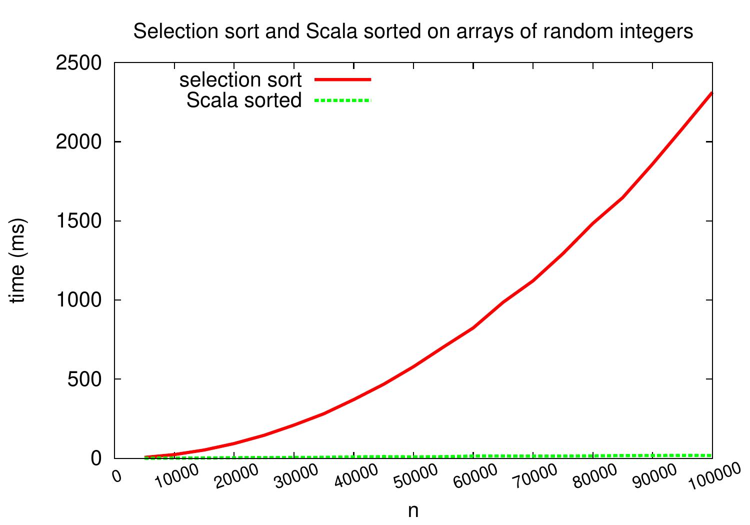
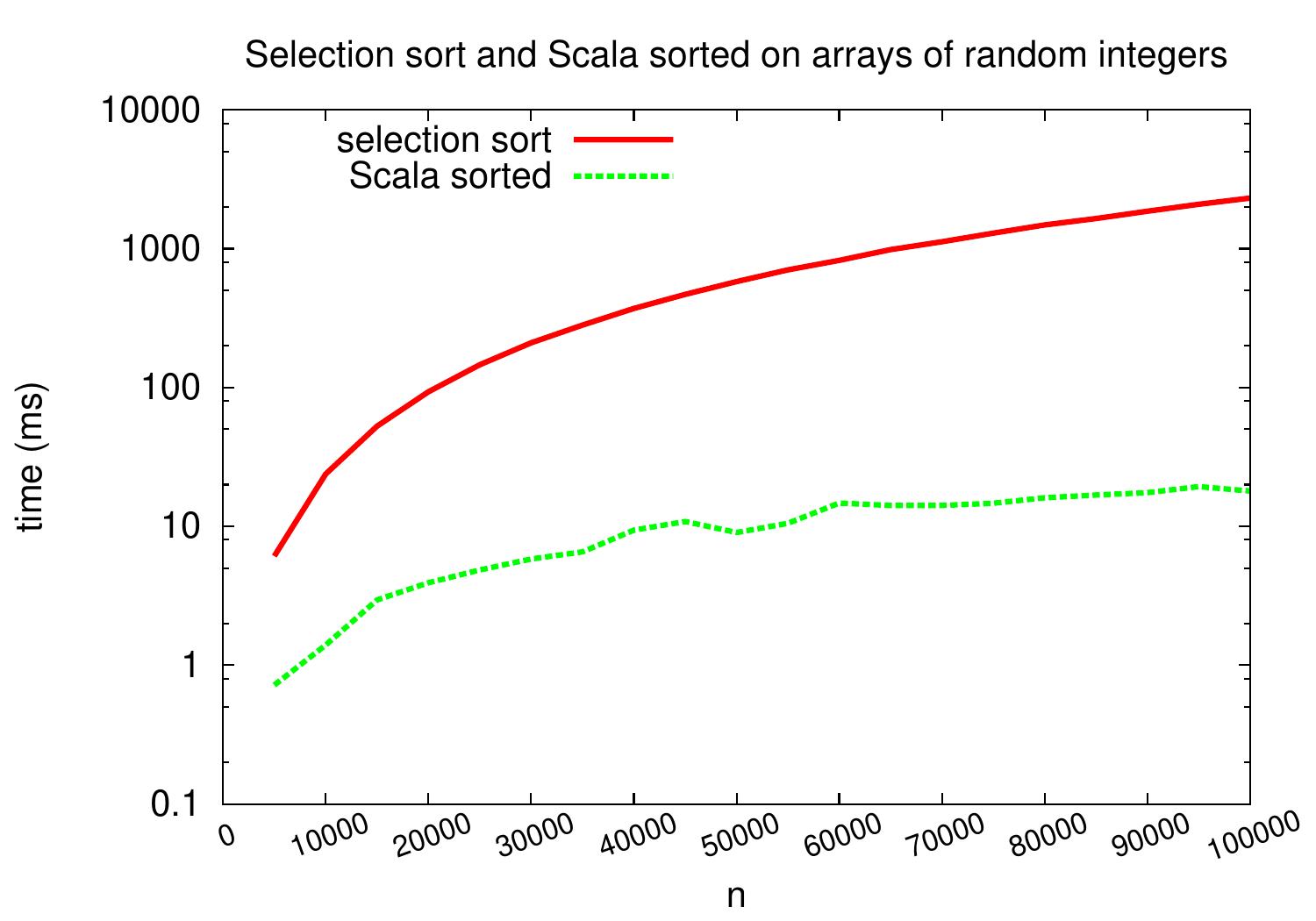
The plots below shows the performance of the above Scala selection sort code when compared to the sorted method of the Array class. When inspecting the latter plot having logarithmic y-axis, we can see that the gap between the lines increases when the array sizes increase. Thus there is more than a constant time factor difference between the running times of the codes. Based on the plots, it is obvious that the sorted method implements an algorithm that scales much better than selection sort.

Generics vs fixed types¶

By using generics (see also this, this and this), it is easy to build a generic selection sort implementation that works for any comparable object type (floating point numbers, strings etc). Using an Ordering ord for the array elements, we only have to change two lines in the code: the method declaration and the comparison line.

def selectionSort[A](a: Array[A])(implicit ord: math.Ordering[A]): Unit = {
  val n = a.length
  var i = 0
  while(i < n-1) {
    // Find the smallest element in the sub-array a(i..n-1)
    var smallest_element = a(i)
    var smallest_index = i
    var j = i + 1
    while(j < n) {
      if(ord.lt(a(j), smallest_element)) {  // CHANGED
	smallest_element = a(j)
	smallest_index = j
      }
      j += 1
    }
    // Swap the elements at a(i) and a(smallest_index)
    a(smallest_index) = a(i)
    a(i) = smallest_element
    // The sub-array a(0..i) is now sorted
    i += 1
  }
}

Unfortunately, with current Scala compiler, the generality does not come without a performance penalty. As an example, consider applying the generic selection sort to arrays of integers. To apply the lt comparison method in the Ordering trait, each integer fetched from the array is “boxed” (wrapped into an object), causing a memory allocation and then later garbage collection. In addition, several virtual function invocations are performed. 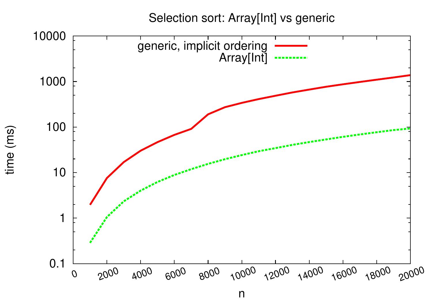We can see the practical effect of this by comparing the running times of our first selection sort working only on integer arrays to those of the generic selection sort algorithm above.

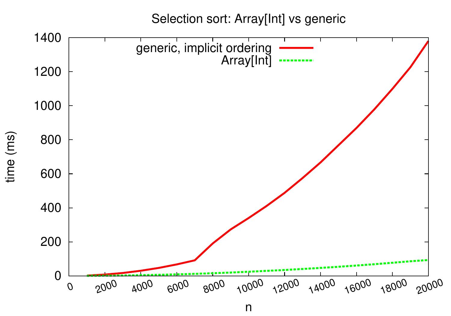
If we use logarithmic scale on the \( y \)-axis, we can see that the running times of the generic version are a constant factor (of roughly ten) slower than those of the non-generic integer array version.