Basic definitions¶

In this round, we study algorithms for sorting sequences, usually arrays, of elements. We assume that a sorting algorithm receives an input array to be sorted, and then rearranges the elements in the same array so that they are in ascending order. That is, the original input array gets modified. For instance, the Java.util.Arrays.sort methods and the C++ standard library sort function work in this way. On the contrary, in Scala the sorted method on sequences does not modify the original array but returns a new array containing the ordered sequence. Under the hood however, it allocates an auxiliary array and applies the Java.util.Arrays.sort function on that copy (see the source code).

For the sake of illustration simplicity, we usually use arrays of integers in the examples. In this case, the elements are sorted by using the usual numeric ascending order \( \le \). For example, an array 7,2,11,5,7 of five integers is sorted into 2,5,7,7,11. Observe that an array can contain multiple equal elements as just illustrated.

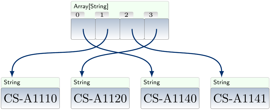
However, one should keep in mind that most of the algorithms extend in a straightforward way to arrays of other types of primitive (integer, floating point number etc) or non-primitive types (strings, pairs, unbounded integers such as Scala BigInt, generic objects) as well. If the elements are non-primitive data types, then in the current version of Java, and thus also in Scala, the sequence contains references to the actual objects, making the swapping of the positions of two objects in the array cheap as one only has to move the references. For instance, swapping the positions of the strings “CS-A1110” and “CS-A1140” in the array

results in the array

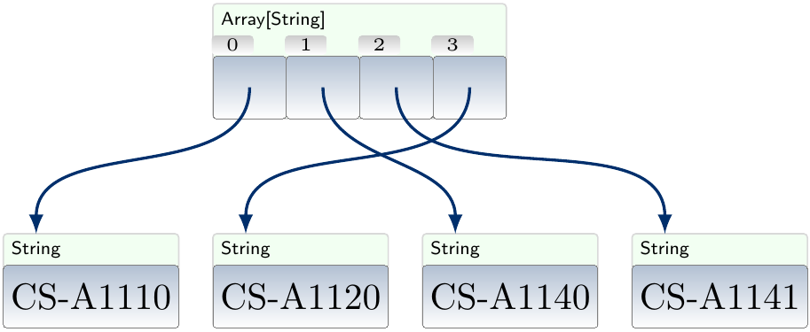
In some other languages, such as C and C++, non-primitive objects can be stored inside the sequences as well. In such a case, swapping the positions of two objects may be more costly.

For all kinds of elements, most sorting algorithms allow the ordering between the elements to be given as input as well. For instance, in Scala we could sort a sequence of floating point numbers into descending order as follows:

scala> val a = Array(1.0,-3.5,5.0,-11.2,24.0)
a: Array[Double] = Array(1.0, -3.5, 5.0, -11.2, 24.0)

scala> a.sortWith(_ > _)
res0: Array[Double] = Array(24.0, 5.0, 1.0, -3.5, -11.2)

Above, the anonymous function _ > _ serves as the less-than ordering argument of the sortWith method. As the result, the sorting algorithm sorts the elements in the ascending order as usual but now the order it considers makes it think that “\( x < y \)” when actually \( x > y \).

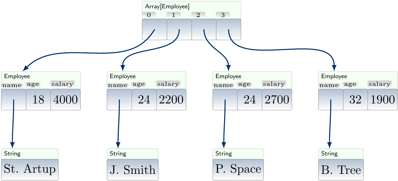
Structured objects can also be sorted with respect to some specific field or substructure called the key. For instance, below the employees are sorted by their age. Note that, again, two distinct objects can be considered equal with respect to the key.

In the running time analyses of sorting algorithms, we assume that random access, meaning reading and writing an element at any position, in the sequence can be done in constant time. Furthermore, for simplicity, we assume that comparing two elements with respect to the applied element ordering can be done in constant time as well. For non-primitive data type objects, such as long strings or complex structured data fields, this may not be the case. In such cases, one could also consider other efficiency aspects such as the numbers of comparisons performed by the algorithms.

Stability¶

Definition: Stable sorting algorithm

A sorting algorithm is stable if it keeps the relative order of equal elements unchanged.

In Scala, the sorted and sortWith methods of sequences implementing SeqLike, such as List and Array, are stable. In addition, sortBy is implemented by using sorted and is also stable.

As an example, we can sort a list

val l = List(("c",2),("b",3),("e",2),("a",3),("b",2),("a",2))

to lexicographical order (first field more significant) by first sorting by the second field

scala> val tmp = l.sortBy(_._2)
tmp = List((c,2), (e,2), (b,2), (a,2), (b,3), (a,3))

and then by the first field with a stable sorting algorithm

scala> val result = tmp.sortBy(_._1)
result = List((a,2), (a,3), (b,2), (b,3), (c,2), (e,2))

In the last step, a stable sorting algorithm keeps the relative order of (a,2) and (a,3) unchanged even though their first fields are the same.

In Java, the java.util.Arrays.sort methods for arrays of objects are stable.

The C++ algorithm library includes separate functions implementing

stable sorting (the stable_sort function), and
sorting that is not quaranteed to be stable (the sort function).

The latter has a slightly better asymptotic worst-case performance in the case there is not enough available memory for an auxiliary array.

Extra memory requirements and in-place sorting¶

Different sorting algorithms also vary in how much extra memory they need during their operation.

Definition

A sorting algorithm needs \( g(n) \) units of extra memory if, when sorting any sequence of length \( n \), the maximum amount of extra memory needed is \( g(n) \). The input/output sequence memory is not counted in \( g(n) \).

As we are usually not interested in the exact amount of extra memory needed but in the growth rate of the extra memory requirements when the input size grows, we use the \( \BigOh \) and \( \Theta \) notations here as well. For instance, some sorting algorithms only use a constant \( \Theta(1) \) amount of extra memory and may thus be very well suited for embedded systems with a limited amount of RAM. On the other hand, some sorting algorithms use \( \Theta(n) \) amount of extra memory because they allocate an auxiliary array of \( n \) elements for computing some intermediate results; this may be justified when both stability and quite good performance are required at the same time.

In addition to the asymptotic extra memory requirement analysis, one regularly also encounters the concept of sorting “in place”. For instance, the following definition is used in the book Introduction to Algorithms, 3rd ed. (online via Aalto lib):

Definition: In-place sorting algorithm

A sorting algorithm works in place if only a constant amount of the array elements are stored outside the array at any moment of time.

The definition above is quite liberal, allowing, for instance, the use of a linear amount of array indices in the recursive call stack of the algorithm. Stricter versions do exist, see, for instance, this Wikipedia page for discussion.