Quicksort¶

Quicksort is another widely used sorting algorithm. Like mergesort, it is a divide and conquer algorithm. Unlike mergesort, it does not need an auxiliary array during sorting and thus needs less memory. Quicksort was published already in 1961

C. A. R. Hoare: Algorithm 63: partition. Communications of the ACM 4(7):321, 1961.
C. A. R. Hoare: Algorithm 64: Quicksort. Communications of the ACM 4(7):321, 1961.

but is still widely used nowadays as well. For instance,

java.util.Arrays.sort on primitive type arrays uses a variant of quicksort, and
the C++ sort uses introsort, which performs quicksort in its first phase.

The basic idea for sorting a sub-array \( A[\LO..\HI] \), with \( \LO \le \HI \), can be described as follows:

Base case: if \( \LO = \HI \), then the sub-array \( A[\LO..\HI] \) has only one element and is thus sorted.
Divide: select a pivot element \( p \) in \( A[\LO..\HI] \), and partition the sub-array \( A[\LO..\HI] \) into three sub-arrays \( A[\LO..q-1] \), \( A[q] \) and \( A[q+1..\HI] \) such that
- all the elements in \( A[\LO..q-1] \) are less than or equal to \( p \),
- \( A[q] = p \), and
- all the elements in \( A[q+1..\HI] \) are greater than \( p \).
After this step, the element \( p \) is in the correct place.
Conquer: recursively sort the sub-arrays \( A[\LO..q-1] \) and \( A[q+1..\HI] \) with quicksort.

The main recursive function, shown below in Scala, is again quite simple:

def quicksort(a: Array[Int]): Unit = {
  // The inner recursive function
  def _quicksort(lo: Int, hi: Int): Unit = {
    // Partition the sub-array a[lo,hi]
    val q = partition(a, lo, hi)
    // Now the element at the index q is in the correct place
    // If the left sub-array has at least two elements, sort it recursively
    if (lo < q - 1)
      _quicksort(lo, q - 1)
    // If the right sub-array has at least two elements, sort it recursively
    if (q + 1 < hi)
      _quicksort(q + 1, hi)
  }
  if (a.length >= 2)
    _quicksort(0, a.length - 1)
}

Example: Sorting an array with quicksort

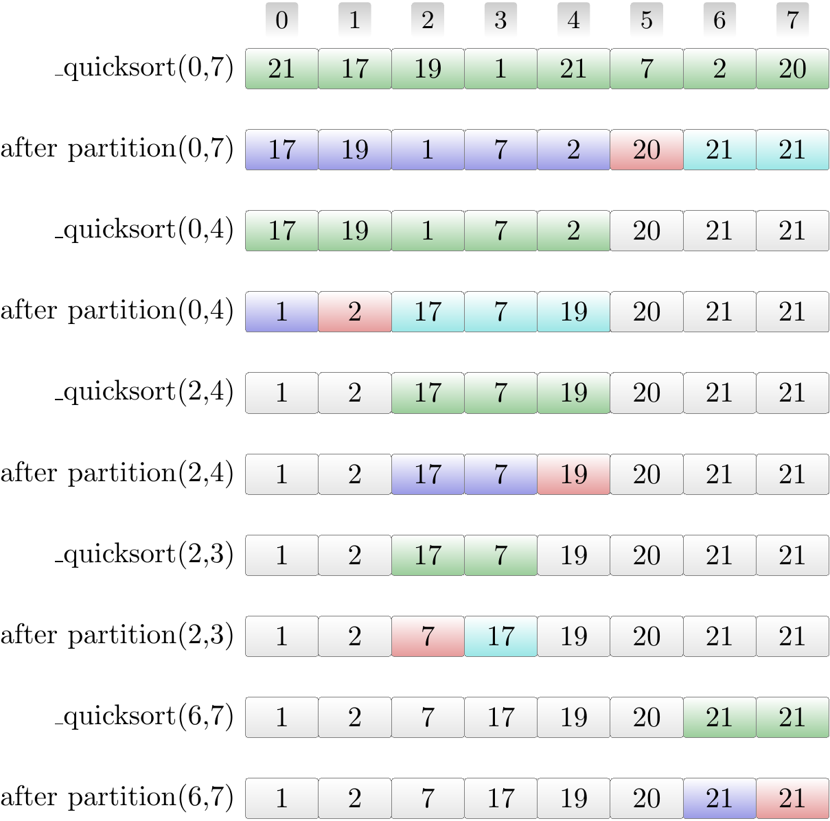
Consider the basic version shown above in Scala. The figure below shows the recursive calls and the results after partitioning in the order they are executed.

The green entries show the current sub-array \( A[\LO..\HI] \).
Red highlights the pivot element.
The blue entries form the left sub-array after partitioning.
The cyan entries form the right sub-array after partitioning.

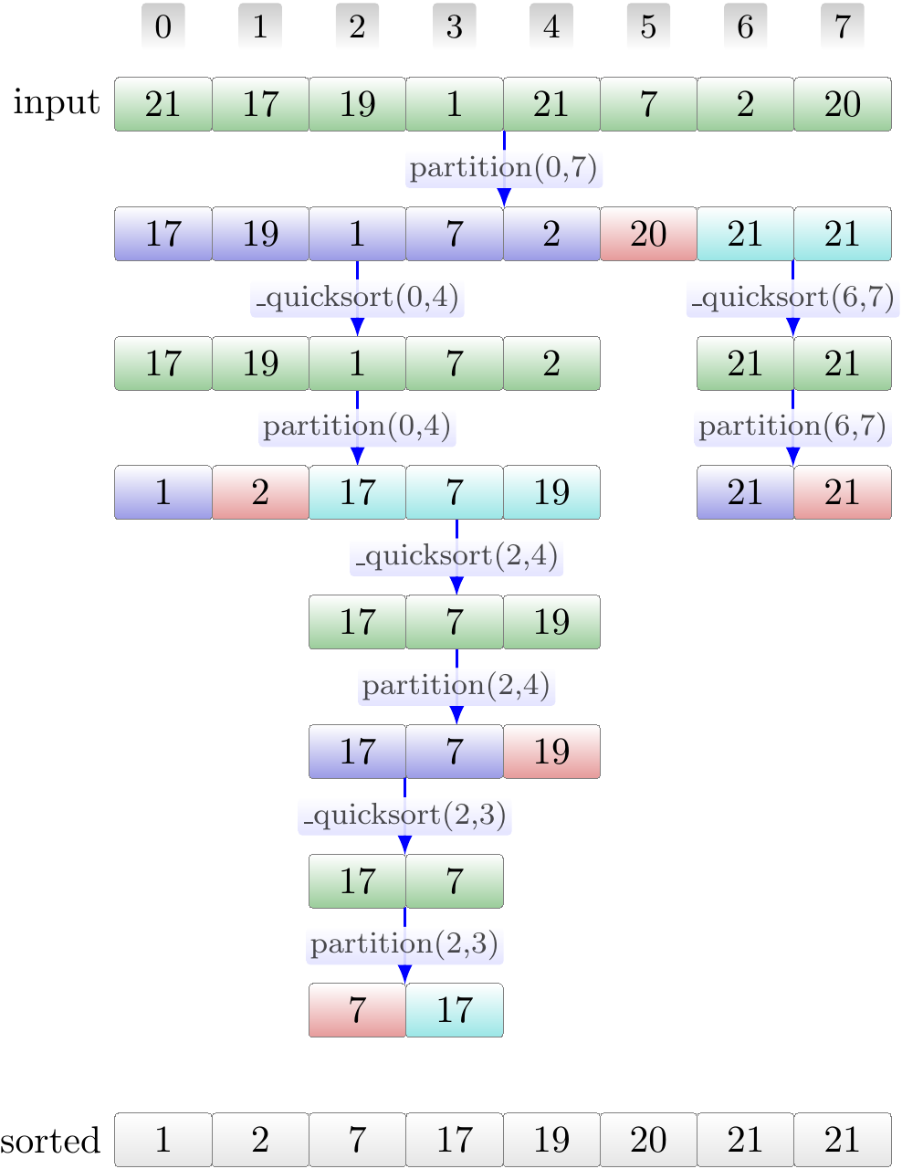
The same in a tree form, showing that, unlike in the case of Mergesort, the recursion tree is not necessarily very well balanced:

In the following, we describe algorithms for performing the partitioning. As we will see, one has to pay attention to the pivot element selection in order to avoid bad worst-case performance of the algorithm.

Lomuto’s partitioning algorithm¶

Lomuto’s partitioning algorithm can be described verbally as follows:

We are given a sub-array \( A[\LO..\HI] \) that we must partition.
We select a pivot element \( p \) occurring in it.
Swap the pivot element with the last element so that it is at the end of the sub-array.
Starting from \( \LO \), maintain two indices \( i \) and \( j \) such that
- the elements left of \( i \) in the sub-array \( A[\LO .. i-1] \) are at most \( p \), and
- the elements from \( i \) until \( j \) are greater than \( p \).
Initially, \( i = \LO \) and \( j = \LO \).
Repeat the following until \( j = \HI \):
- If the element \( A[j] \le p \), swap the elements at the indices \( i \) and \( j \), and increase \( i \) by one.
- Increase \( j \) by one.
Finally, swap the last element (the pivot) with the one at the index \( i \).

Example: Lomuto’s partitioning algorithm

Let’s apply Lomuto’s algorithm to partition a sub-array \( a[2,9] \) shown below. The pivot element has already been selected and moved to be the last element \( a[9] \). The entries will be colored as follows:

Yellow: the pivot element.
Blue: the entries from \( lo \) until \( i \). They are less or equal to the pivot.
Green: the entries from \( i \) until \( j \). The are greater than the pivot.
White: elements outside the sub-array. They are not touched by the algorithm.
Grey: the elements in the sub-array that have not yet been considered.

Click on the image to step the animation.

We can implement the partition algorithm is Scala as follows:

/*
 * An auxiliary helper method.
 * Swap the elements at the indices i and j in the array a.
 */
def swap(a: Array[Int], i: Int, j: Int): Unit = {
  val t = a(i); a(i) = a(j); a(j) = t
}

/*
 * Partition the sub-array a[lo,hi].
 * Return the index of the pivot element in the result.
 */
def partition(a: Array[Int], lo: Int, hi: Int): Int = {
  // Very simple pivot selection, will be improved later!
  val pivot = a(hi)
  // a[lo,i-1] will contain elements less or equal to the pivot
  var i = lo
  // a[i,j-1] will contain elements greater than the pivot
  var j = lo
  while(j < hi) {
    if(a(j) <= pivot) {
      swap(a, i, j)
      i += 1
    }
    j += 1
  }
  // Move the pivot element into its correct place
  swap(a, i, hi)
  // Return the index of the pivot element
  i
}

Instability¶

Quicksort, as presented above, is not stable because the partitioning method can change the relative order of elements with the same key. A simple example is shown below.

Example: Instability in Lomuto’s algorithm

The animation shows a partitioning where the relative order of the elements with the key 10 is changed.

Experimental evaluation¶

Let’s compare the practical performance of the mergesort and quicksort algorithm implementations presented in these notes. As inputs, we again use arrays of random integers.

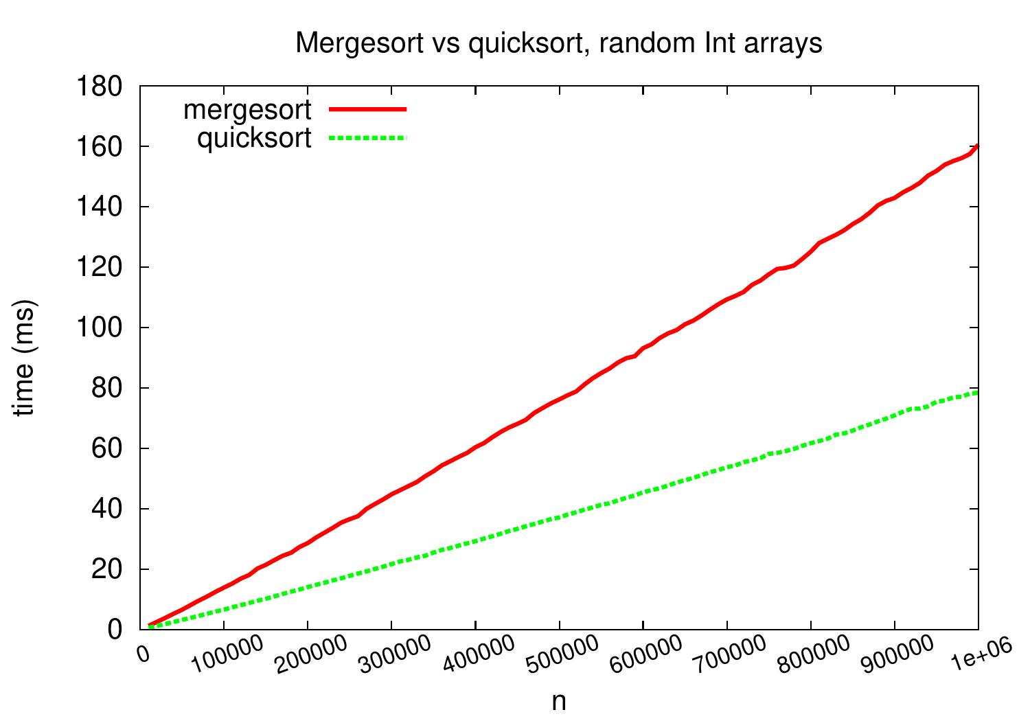
On these implementations and inputs, quicksort is about two times faster.

Let’s further compare the performance of these simple implementations against Scala’s Array[Int].sorted method and the java.util.Arrays.sort method.

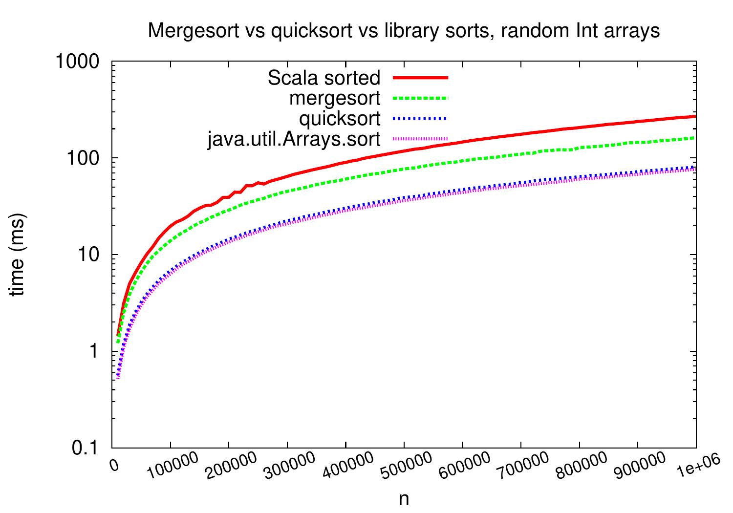
_images/merge-vs-quick-vs-standard-large-logy.jpg

On random integer arrays, our quicksort performs very similarly to java.util.Arrays.sort. Unsurprisingly, the implementation of java.util.Arrays.sort in this case is a variant of quicksort (see, for instance, this source code). Currently, the Array[Int].sorted method maps integers into objects and uses java.util.Arrays.sort for objects, which currently implements the TimSort algorithm (source code).

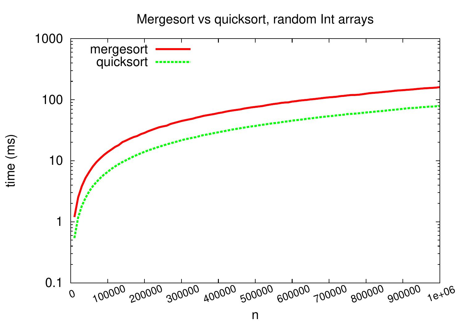
Analysis and improvements¶

Based on the above experimental plots, our quicksort algorithm seems to be an \( \Oh{n \Lg{n}} \) algorithm as it scales similarly to mergesort. However, this is not the case: in the worst case, the basic version takes \( \Theta(n^2) \) time as argued below.

Partitioning takes \( \Theta(k) \) time, where \( k \) is the length of the considered sub-array.
In our basic version, we select the last element in the sub-array to be the pivot element.
The quadratic-time worst case perfomance occurs when the array is already sorted:
- The pivot element does not move anywhere and we effectively just produce one partition of size \( k-1 \).
- Thus the recurrence is \( T(n) = \Theta(n) + T(n-1) = \Theta(n^2) \).

The Scala version presented above does not actually work at all on large already sorted arrays because the recursion depth is also large and one gets a stack overflow error.

Pivot selection¶

The quadratic time consumption on already sorted data is not desirable as in practise it can be quite common that the data is already almost in order. Therefore, pivot element selection is important.

Worst-case \( \Oh{n \Lg n} \) run-time is obtained when the pivot is chosen so that the obtained two partitions are of roughly equal size. Thus one could choose the pivot to be the median of the subarray considered. In principle, the median can be computed in linear time, see Section 9.3 in Introduction to Algorithms, 3rd ed. (online via Aalto lib), but the constant factors in this operation are quite large. A practical approximation is to select the pivot to be the median of three random elements in the subarray. Another common and easy-to-implement strategy is to select a random element in the subarray to be the pivot element. After the selection, the pivot is moved to be the last element and we then proceed as earlier in the partition algorithm. For arrays with \( n \) distinct elements, the expected run-time of quicksort is \( \Oh{n \Lg{n}} \) when random pivots are chosen, see Section 7.4 in Introduction to Algorithms, 3rd ed. (online via Aalto lib). This is what happened in our experiments above: we did not choose random pivots but the elements were random and thus the situation was effectively the same.

Multiple equal elements¶

Pivot selection does not help when the array has a lot of equal elements. Consider the case that the array consists of \( n \) elements that are all the same. No matter how the pivot is selected, the partitioning of a subarray with \( k \) elements again effectively produces just one partition with \( k-1 \) elements that are the same as the pivot element. Thus the running time of the basic quicksort algorithm is again \( \Theta(n^2) \). This problem can be solved by using a partitioning function that produces three partitions:

one with elements smaller than the pivot element,
one with elements equalt to the pivot element (including the pivot element itself), and
one with elements larger than the pivot.

The partition with equal elements needs not to be further processed as it is already sorted. The implementation of this three-way partitioning algorithm is left as a programming exercise.

Hoare’s partitioning algorithm¶

The partition algorithm presented above is not the original one published by Sir Tony Hoare in 1962 (see the original article). Like Lomuto’s algorithm, the original one uses two indices \( i \) and \( j \) but they start scanning the sub-array from the beginning and the end, respectively. A version of the algorithm can be described verbally as follows:

As earlier, the input is a sub-array \( A[\LO .. \HI] \) with at least two elements.
Select a pivot element \( p \) in the sub-array.
Swap the pivot element with the last one so that it is at the end of the sub-array.
Maintain indices \( i \) and \( j \), initially \( i=\LO \) and \( j = \HI \), so that
- the elements at \( \LO,…,i-1 \) are at most \( p \)
- the elements at \( j+1,…,\HI-1 \) are greater than \( p \)
Repeat until \( i > j \)
- Until \( i \) is equal to \( j \) or \( A[i] > p \), increase the value of \( i \)
- Decrease the value of \( j \) until it is equal to \( i \) or \( A[j] \le p \)
- If \( i < j \), swap the elements at indices \( i \) and \( j \)
Finally, swap the last element (the pivot) with the one in index \( i \)

Example: Hoare’s partitioning algorithm

Let’s apply Hoare’s algorithm to partition a sub-array \( a[2,9] \) shown below. The pivot element has already been selected and moved to be the last element \( a[9] \). The entries will be colored as follows:

Yellow: the pivot element.
Blue: the entries found to be less or equal to the pivot.
Green: the entries found to be greater than the pivot.
White: elements outside the sub-array. They are not touched by the algorithm.
Grey: the elements in the sub-array that have not yet been considered.

Click on the image to step the animation.

An implementation in Scala:

def swap(a: Array[Int], i: Int, j: Int): Unit = {
  val t = a(i); a(i) = a(j); a(j) = t
}

def partition(a: Array[Int], lo: Int, hi: Int): Int = {
  val pivot = a(hi)  // Very simple pivot selection!
  var i = lo
  var j = hi
  while(i <= j) {
    while(i < j && a(i) <= pivot) {
      i = i + 1
    }
    do {
      j = j - 1
    } while (i <= j && a(j) > pivot)
    if(i < j)
      swap(a, i, j)
  }
  swap(a, hi, i)
  i
}

The practical performance is similar to that of Lomuto’s algorithm.

Using Hoare’s partitioning algorithm also produces an instable quicksort sorting algorithm — can you find a simple example illustrating why this is the case?