Insertion sort¶

Insertion sort is another elementary sorting algorithm whose algorithmic idea is rather easy to understand. However, as we’ll see, it can be considered efficient only for small arrays. The algorithmic idea of insertion sort can be stated as follows:

Assume that the sub-array with the first \( i \) elements of the array is already sorted. In the first round, \( i = 1 \).
Take the \( i+1 \):th element \( e \). Shift the last elements in the sorted sub-array prefix one step right until the correct position for \( e \) is reached. Insert \( e \) to that position.
Now the sub-array of the first \( i+1 \) elements is sorted.
Repeat until the whole array is sorted.

In pseudocode, insertion sort can be described as follows. Please notice that, unlike in Introduction to Algorithms, 3rd ed. (online via Aalto lib), we start array indexing from \( 0 \), not from \( 1 \).

Insertion-sort(\( A \)):
  for \( i \Asgn 1 \) until \( \ALengthOf{A} \):
    \( e \Asgn A[i] \)    // element to be moved
    \( j \Asgn i \)
    while \( j > 0 \) and \( A[j-1] > e \):
      \( A[j] \Asgn A[j-1] \)
      \( j \Asgn  j-1 \)
    \( A[j] \Asgn e \)
 

An implementation for integer arrays in Scala looks quite similar:

def insertionSort(a: Array[Int]): Unit = {
  var i = 1
  while (i < a.length) {
    val key = a(i)
    var j = i;
    while (j > 0 && a(j - 1) > key) {
      a(j) = a(j - 1)
      j -= 1
    }
    a(j) = key
    i += 1
  }
}

Example: Insertion sort

The animation below shows how selection sort works on a smallish array of integers. The sorted sub-array is shown in blue.

Some properties of the algorithm:

Only the element currently moved is stored outside the array at any point of time. Thus the amount of extra memory required is \( \Theta(1) \) and the algorithm works in place.
It is stable because we always find the rightmost position where the currently considered element belongs to, meaning that it is never moved left past an equal element.

Running time analysis¶

In the following analyses it is assumed that both (i) the comparison of two elements, as well as (ii) the array accesses are constant-time operations.

In the best case, insertion sort runs in time \( \Theta(n) \). To see this, consider how the algorithm behaves on arrays that are already sorted. In such arrays, in each round, the next element considered is already at its correct position and this can be detected by using just one comparison and no shifts.

In the worst case, the running time of the algorithm is \( \Theta(n^2) \). To see this, consider an array of \( n \) distinct elements that is sorted in reverse order. Now

the second element is moved 1 steps,
the third element is moved 2 steps,
and so on, and
the \( n \):th element is moved \( n-1 \) steps.

Each move of \( i \) steps induces the same amount of shifts. Therefore, at the \( i \)th round the algorithm performs \( \Theta(i) \) comparisons and array accesses. Thus the running time recurrence is \( T(n) = \Theta(n) + T(n-1) = \Theta(n^2) \).

What about average case performance? Consider an array consisting of \( n \) distinct random elements. At each iteration, when moving the \( i \)th element \( a_i \) to its correct position, there are on average \( i/2 \) elements in the sub-array \( \Arr{a_0,…,a_{i-1}} \) that are smaller than \( a_i \). Therefore, the work on average is \( \sum_{i=1}^{n-1} i/2 = \Theta(n^2) \).

How about the performance on a specific application? This depends on the inputs that the application provides. If the input is usually almost sorted already, insertion sort may work fine in practise. But if the inputs are usually in random order or in some order causing \( \Oh{n} \) elements to be moved long distances, we should probably consider some other algorithm.

Observe that insertion sort code is very “compact” (small constants) and the memory accesses are very local. Therefore, for small arrays, insertion sort can be quite competitive as we will see later.

If the key comparisons are expensive, one could use binary search for finding the correct place for each insertion. The causes number of comparisons to drop to \( \Oh{n \Lg n} \) in the worst case. But the overall running time stays \( \Theta(n^2) \) as the shifts still need to be performed.

Experimental evaluation¶

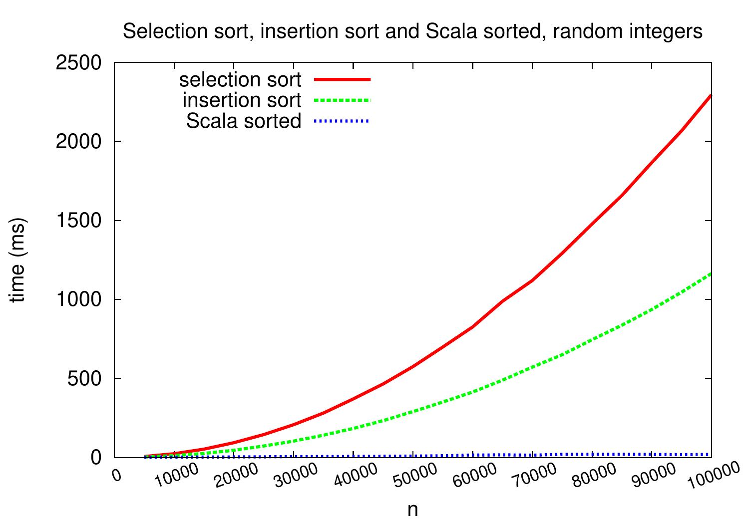
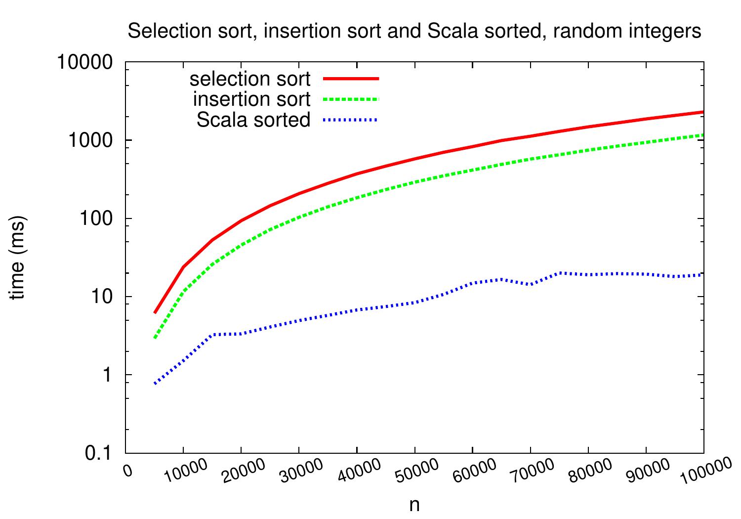
The plots below show the performance of the above Scala implementation of insertion sort with respect to selection sort (Section Selection sort) and the sorted method of the Scala Array class. As we can see, insertion sort is roughly twice as fast as selection sort on these input arrays consisting of random integers. However, their performance scales similarly and they are not that efficient as the algorithm in the sorted method on these inputs.