\(\) \(%\newcommand{\CLRS}{\href{https://mitpress.mit.edu/books/introduction-algorithms}{Cormen et al}}\) \(\newcommand{\CLRS}{\href{https://mitpress.mit.edu/books/introduction-algorithms}{Introduction to Algorithms, 3rd ed.} (\href{http://libproxy.aalto.fi/login?url=http://site.ebrary.com/lib/aalto/Doc?id=10397652}{online via Aalto lib})}\) \(\newcommand{\SW}{\href{http://algs4.cs.princeton.edu/home/}{Algorithms, 4th ed.}}\) \(%\newcommand{\SW}{\href{http://algs4.cs.princeton.edu/home/}{Sedgewick and Wayne}}\) \(\) \(\newcommand{\Java}{\href{http://java.com/en/}{Java}}\) \(\newcommand{\Python}{\href{https://www.python.org/}{Python}}\) \(\newcommand{\CPP}{\href{http://www.cplusplus.com/}{C++}}\) \(\newcommand{\ST}[1]{{\Blue{\textsf{#1}}}}\) \(\newcommand{\PseudoCode}[1]{{\color{blue}\textsf{#1}}}\) \(\) \(%\newcommand{\subheading}[1]{\textbf{\large\color{aaltodgreen}#1}}\) \(\newcommand{\subheading}[1]{\large{\usebeamercolor[fg]{frametitle} #1}}\) \(\) \(\newcommand{\Blue}[1]{{\color{flagblue}#1}}\) \(\newcommand{\Red}[1]{{\color{aaltored}#1}}\) \(\newcommand{\Emph}[1]{\emph{\color{flagblue}#1}}\) \(\) \(\newcommand{\Engl}[1]{({\em engl.}\ #1)}\) \(\) \(\newcommand{\Pointer}{\raisebox{-1ex}{\huge\ding{43}}\ }\) \(\) \(\newcommand{\Set}[1]{\{#1\}}\) \(\newcommand{\Setdef}[2]{\{{#1}\mid{#2}\}}\) \(\newcommand{\PSet}[1]{\mathcal{P}(#1)}\) \(\newcommand{\Card}[1]{{\vert{#1}\vert}}\) \(\newcommand{\Tuple}[1]{(#1)}\) \(\newcommand{\Implies}{\Rightarrow}\) \(\newcommand{\Reals}{\mathbb{R}}\) \(\newcommand{\Seq}[1]{(#1)}\) \(\newcommand{\Arr}[1]{[#1]}\) \(\newcommand{\Floor}[1]{{\lfloor{#1}\rfloor}}\) \(\newcommand{\Ceil}[1]{{\lceil{#1}\rceil}}\) \(\newcommand{\Path}[1]{(#1)}\) \(\) \(%\newcommand{\Lg}{\lg}\) \(\newcommand{\Lg}{\log_2}\) \(\) \(\newcommand{\BigOh}{O}\) \(%\newcommand{\BigOh}{\mathcal{O}}\) \(\newcommand{\Oh}[1]{\BigOh(#1)}\) \(\) \(\newcommand{\todo}[1]{\Red{\textbf{TO DO: #1}}}\) \(\) \(\newcommand{\NULL}{\textsf{null}}\) \(\) \(\newcommand{\Insert}{\ensuremath{\textsc{insert}}}\) \(\newcommand{\Search}{\ensuremath{\textsc{search}}}\) \(\newcommand{\Delete}{\ensuremath{\textsc{delete}}}\) \(\newcommand{\Remove}{\ensuremath{\textsc{remove}}}\) \(\) \(\newcommand{\Parent}[1]{\mathop{parent}(#1)}\) \(\) \(\newcommand{\ALengthOf}[1]{{#1}.\textit{length}}\) \(\) \(\newcommand{\TRootOf}[1]{{#1}.\textit{root}}\) \(\newcommand{\TLChildOf}[1]{{#1}.\textit{leftChild}}\) \(\newcommand{\TRChildOf}[1]{{#1}.\textit{rightChild}}\) \(\newcommand{\TNode}{x}\) \(\newcommand{\TNodeI}{y}\) \(\newcommand{\TKeyOf}[1]{{#1}.\textit{key}}\) \(\) \(\newcommand{\PEnqueue}[2]{{#1}.\textsf{enqueue}(#2)}\) \(\newcommand{\PDequeue}[1]{{#1}.\textsf{dequeue}()}\) \(\) \(\newcommand{\Def}{\mathrel{:=}}\) \(\) \(\newcommand{\Eq}{\mathrel{=}}\) \(\newcommand{\Asgn}{\mathrel{\leftarrow}}\) \(%\newcommand{\Asgn}{\mathrel{:=}}\) \(\) \(%\) \(% Heaps\) \(%\) \(\newcommand{\Downheap}{\textsc{downheap}}\) \(\newcommand{\Upheap}{\textsc{upheap}}\) \(\newcommand{\Makeheap}{\textsc{makeheap}}\) \(\) \(%\) \(% Dynamic sets\) \(%\) \(\newcommand{\SInsert}[1]{\textsc{insert}(#1)}\) \(\newcommand{\SSearch}[1]{\textsc{search}(#1)}\) \(\newcommand{\SDelete}[1]{\textsc{delete}(#1)}\) \(\newcommand{\SMin}{\textsc{min}()}\) \(\newcommand{\SMax}{\textsc{max}()}\) \(\newcommand{\SPredecessor}[1]{\textsc{predecessor}(#1)}\) \(\newcommand{\SSuccessor}[1]{\textsc{successor}(#1)}\) \(\) \(%\) \(% Union-find\) \(%\) \(\newcommand{\UFMS}[1]{\textsc{make-set}(#1)}\) \(\newcommand{\UFFS}[1]{\textsc{find-set}(#1)}\) \(\newcommand{\UFCompress}[1]{\textsc{find-and-compress}(#1)}\) \(\newcommand{\UFUnion}[2]{\textsc{union}(#1,#2)}\) \(\) \(\) \(%\) \(% Graphs\) \(%\) \(\newcommand{\Verts}{V}\) \(\newcommand{\Vtx}{v}\) \(\newcommand{\VtxA}{v_1}\) \(\newcommand{\VtxB}{v_2}\) \(\newcommand{\VertsA}{V_\textup{A}}\) \(\newcommand{\VertsB}{V_\textup{B}}\) \(\newcommand{\Edges}{E}\) \(\newcommand{\Edge}{e}\) \(\newcommand{\NofV}{\Card{V}}\) \(\newcommand{\NofE}{\Card{E}}\) \(\newcommand{\Graph}{G}\) \(\) \(\newcommand{\SCC}{C}\) \(\newcommand{\GraphSCC}{G^\text{SCC}}\) \(\newcommand{\VertsSCC}{V^\text{SCC}}\) \(\newcommand{\EdgesSCC}{E^\text{SCC}}\) \(\) \(\newcommand{\GraphT}{G^\text{T}}\) \(%\newcommand{\VertsT}{V^\textup{T}}\) \(\newcommand{\EdgesT}{E^\text{T}}\) \(\) \(%\) \(% NP-completeness etc\) \(%\) \(\newcommand{\Poly}{\textbf{P}}\) \(\newcommand{\NP}{\textbf{NP}}\) \(\newcommand{\PSPACE}{\textbf{PSPACE}}\) \(\newcommand{\EXPTIME}{\textbf{EXPTIME}}\)
\(\newcommand{\LO}{{\textit{lo}}}\) \(\newcommand{\HI}{{\textit{hi}}}\)

Counting and Radix Sorts

For some element types, we can do sorting that is not based on direct comparisons. Or in other words, sometimes we can exploit properties of the elements to perform faster sorting. In the following, we consider

  • ​ counting sort that is applicable for some small element sets, and

  • ​ radix sorts that exploit the structure of the elements.

Counting sort

Assume that the set of possible elements is, or is easily mappable to, the set \( \Set{0,…,k-1} \) for some reasonably small \( k \). For instance, if we wish to sort an array of bytes, then \( k = 256 \). Similarly, \( k = 6 \) when sorting the students of a course by their grade. The idea in counting sort is to

  • ​ first count the occurrences of each element in the array, and

  • ​ then use the cumulated counts to indicate where each element should be sorted to.

In pseudo-code, the algorithm can be expressed as follows. The steps in the algorithm will be explained and illustrated in the following example.

counting-sort(\( A \)): // 1: Allocate and initialize auxiliary arrays \( count \Asgn \)int-array of length k \( start \Asgn \)int-array of length k \( result \Asgn \)int-array of length \( \ALengthOf{A} \) for \( v \) in \( 0 \) until \( k \): \( count[v] \Asgn 0 \) // 2: Count occurrences for \( i \) in \( 0 \) until \( \ALengthOf{A} \): \( count[A[i]] \mathop{{+}{=}} 1 \) // 3: Cumulative occurrences: \( start[i] = \sum_{j=0}^{i-1}count[i] \) \( start[0] \Asgn 0 \) for \( j \) in \( 1 \) until \( k \): \( start[j] \Asgn start[j-1] + count[j-1] \) // 4: Make the result for \( i \) in \( 0 \) until \( \ALengthOf{A} \): \( result[start[A[i]]] \Asgn A[i] \) \( start[A[i]] \mathop{{+}{=}} 1 \)

Example: Counting sort

Let’s apply counting sort to an array of octal digits 0,1,…,7.

  • ​ In phase 1, we allocate the auxiliary count and result arrays and initialize the count array with 0s. Takes time \( \Theta(k) \) and here \( k = 8 \).

    _images/countingsort2-1.png
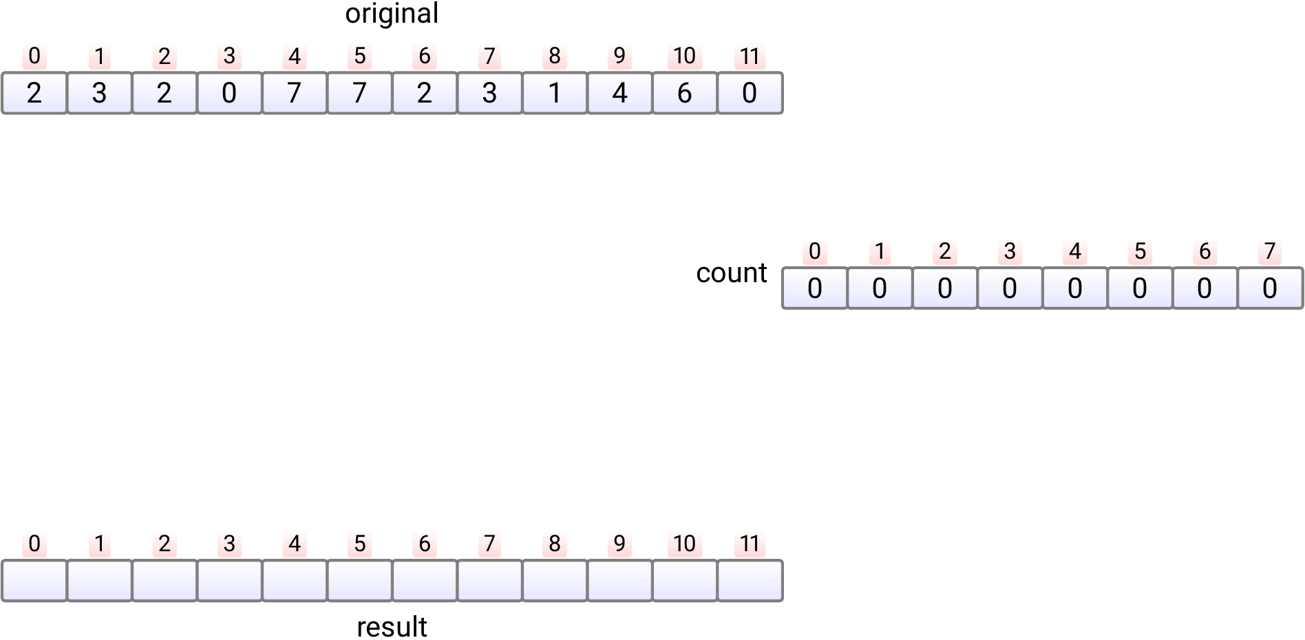
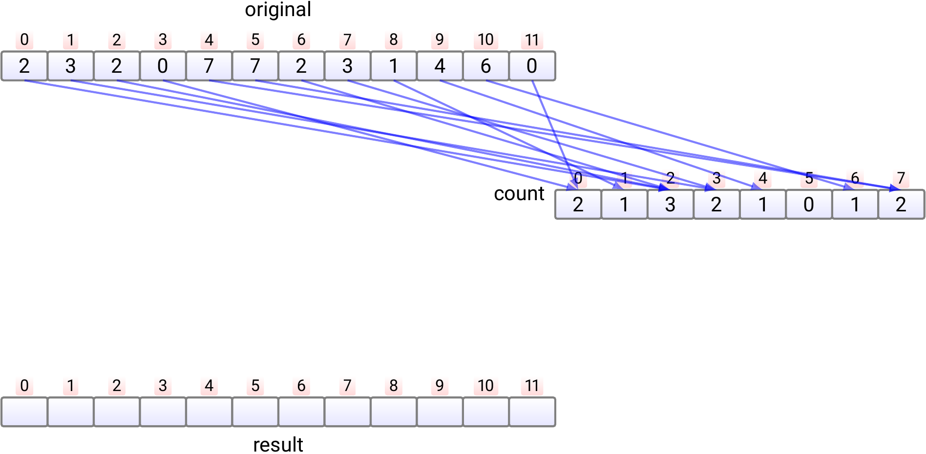
  • ​ In phase 2, we count, in \( n \) steps, in each position \( count[j] \) how many times the element \( j \) occurs in the input array. This phase take time \( \Theta(n) \).
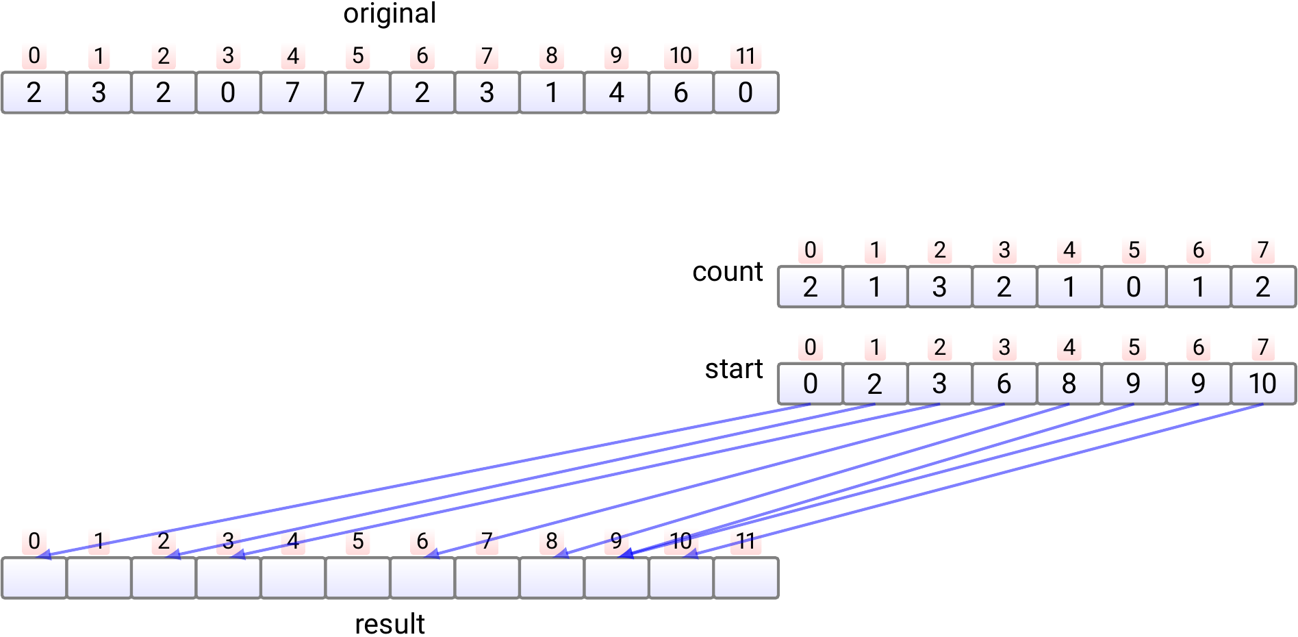
    _images/countingsort2-2.png
  • ​ In phase 3,

    • ​ For each value \( j \), compute \( start[j] = \sum_{l = 0}^{j-1} count[l] \) which tells the position of the first occurrence of the element \( j \) in the sorted result array

    • ​ Takes time \( \Theta(k) \).

    • Note: as we will not use the count after this, we could compute the information of the start array directly into it, saving some memory allocation.

    _images/countingsort2-3.png
  • ​ In phase 4, the elements in the original array are moved, one by one, into the correct position in the result array.

    1. Copy the element \( e_0 \) at index 0 to the index \( start[e_0] \) in the result array. Increment \( start[e_0] \) by one.

      _images/countingsort2-4.png
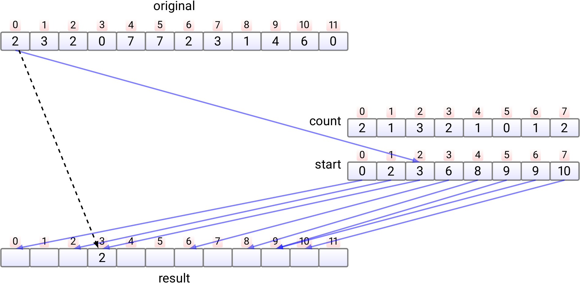
    2. Copy the element \( e_1 \) at index 1 to the index \( start[e_1] \) in the result array. Increment \( start[e_1] \) by one.

      _images/countingsort2-5.png
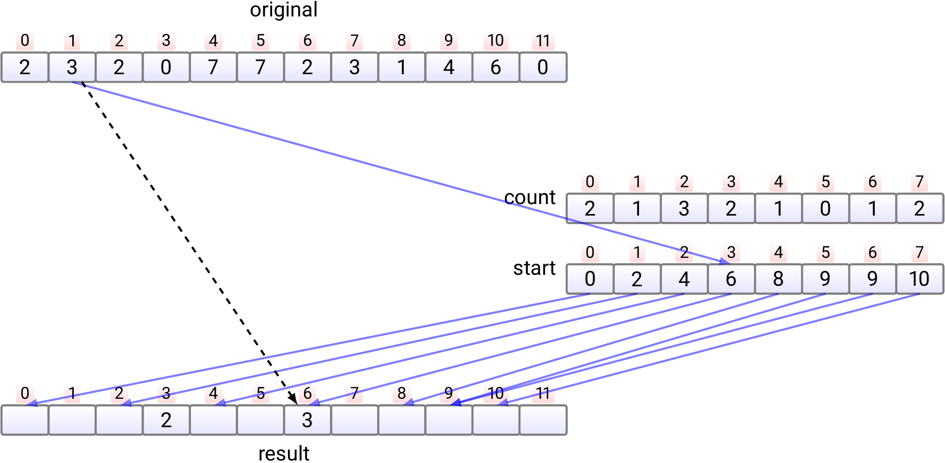
    3. Copy the element \( e_2 \) at index 2 to the index \( start[e_2] \) in the result array. Increment \( start[e_2] \) by one.
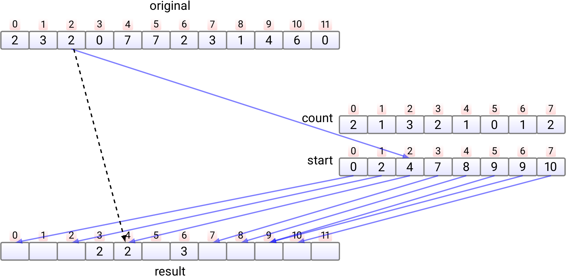
      _images/countingsort2-6.png
    4. And so on.

  • ​ Finally, if needed, copy the sorted array back from the result array to the original array. This phase is not shown in the pseudo-code and is not always required.

    _images/countingsort2-7.png

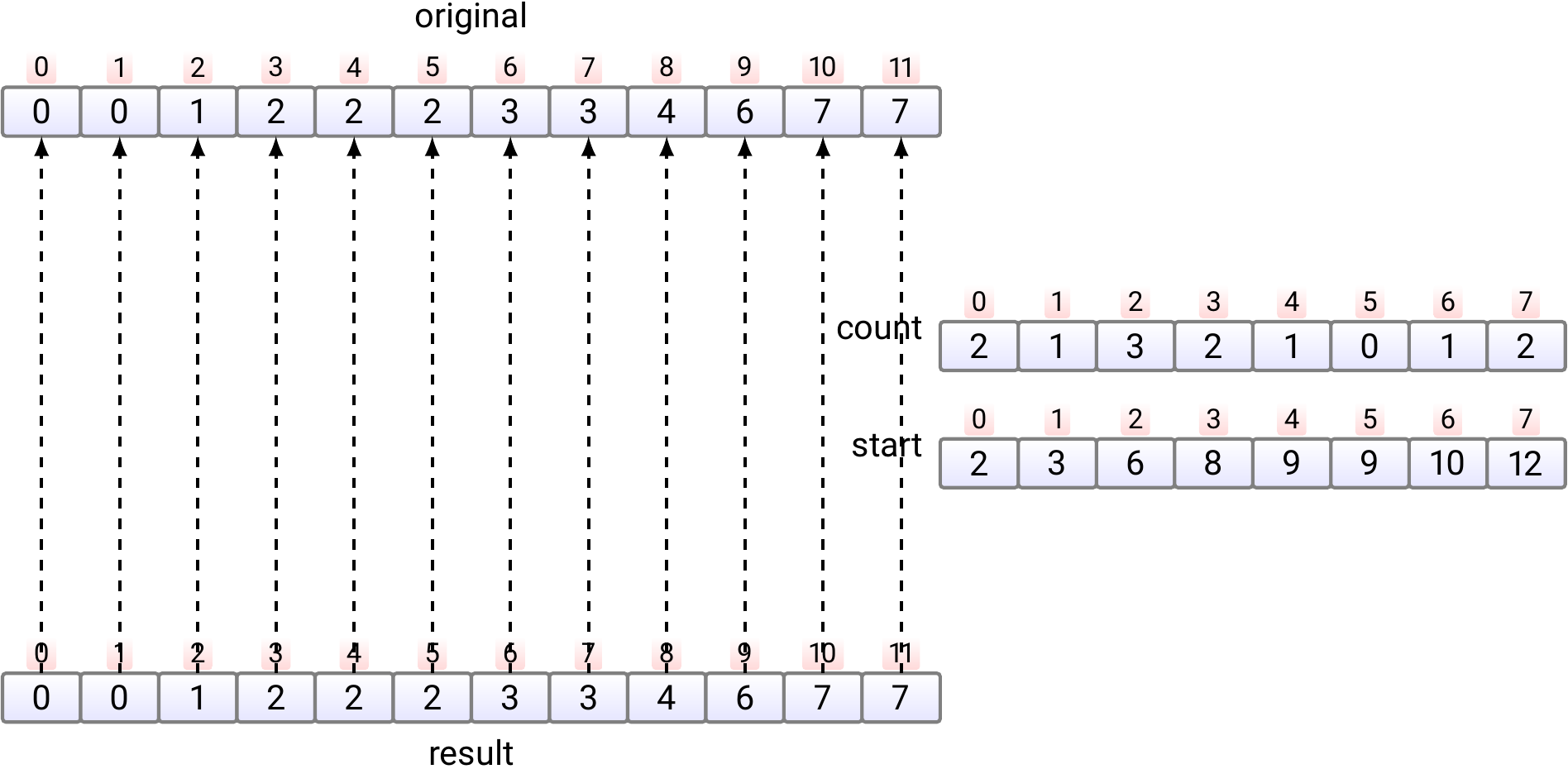
The algorithm uses \( \Theta(n+k) \) amount of extra space and thus does not work “in place”.

Properties:

  • ​ Stable. Why?

  • ​ Needs \( \Theta(k + n) \) extra memory.

  • ​ Works in \( \Theta(k + n) \) time.

  • ​ A very competitive algorithm when \( k \) is small and \( n \) is large.

Most-significant-digit-first radix sort

Assume that

  • ​ the elements are sequences of digits from \( 0,….,k-1 \) and

  • ​ we wish to sort them in lexicographical order.

For instance,

  • ​ 32-bit integers are sequences of length \( 4 \) of \( 8 \)-bit bytes, and

  • ​ ASCII-strings are sequences of ASCII-characters.

The most-significant-digit-first radix sort

  • ​ first sorts the keys according to their first (most significant) digit by using counting sort, and

  • ​ then, recursively, sorts each sub-array that (i) has the same most significant digit and (ii) is of length two or more, by considering sequences starting from the second digit.
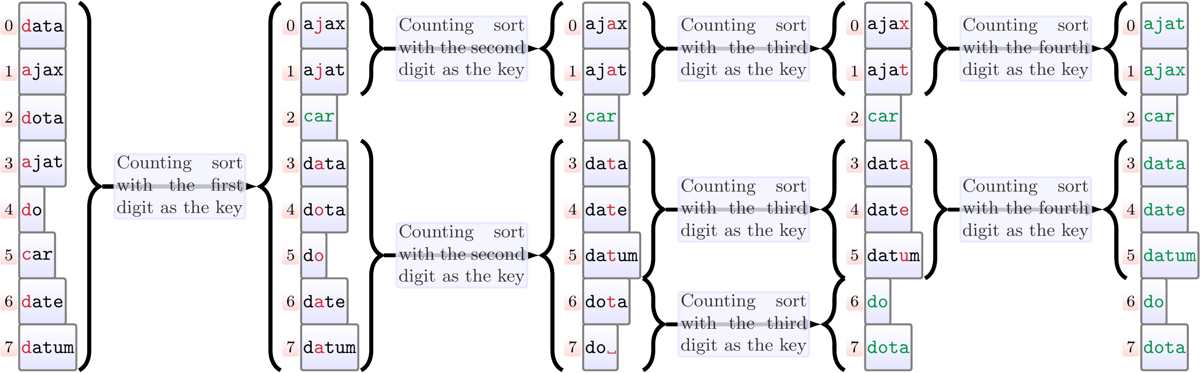
Example

The figure below illustrates the recursive calls done when sorting eight strings with most-significant-digit-first radix sort. As the sequences may not be of the same length, each sequence can be thought to end with a special symbol ␣ that is the smallest digit.

_images/radix-msdf.png

Properties:

  • ​ Stable

  • ​ Needs \( \Theta(k+n+d) \) extra memory, where \( d \) is the maximum length of the sequences

  • ​ Works in \( \BigOh(knd) \) time, where \( d \) is the maximum length of the sequences

Least-significant-digit-first radix sort

Again, assume that the keys are sequences of digits from \( 0,….,k-1 \) and we wish to sort them in lexicographical order. But now also assume that all the keys are of the same length \( d \). For instance, the keys could be

  • ​ 32-bit integers are sequences of length \( 4 \) of \( 8 \)-bit bytes, or

  • ​ ASCII-strings of the same length, such as Finnish social security numbers.

The least-significant-digit-first radix sort

  • ​ first sorts the keys according to their last (least significant) digit by using the stable counting sort, and

  • ​ then, iteratively, sorts the keys according to their second-last digit by using the stable counting sort and so on.
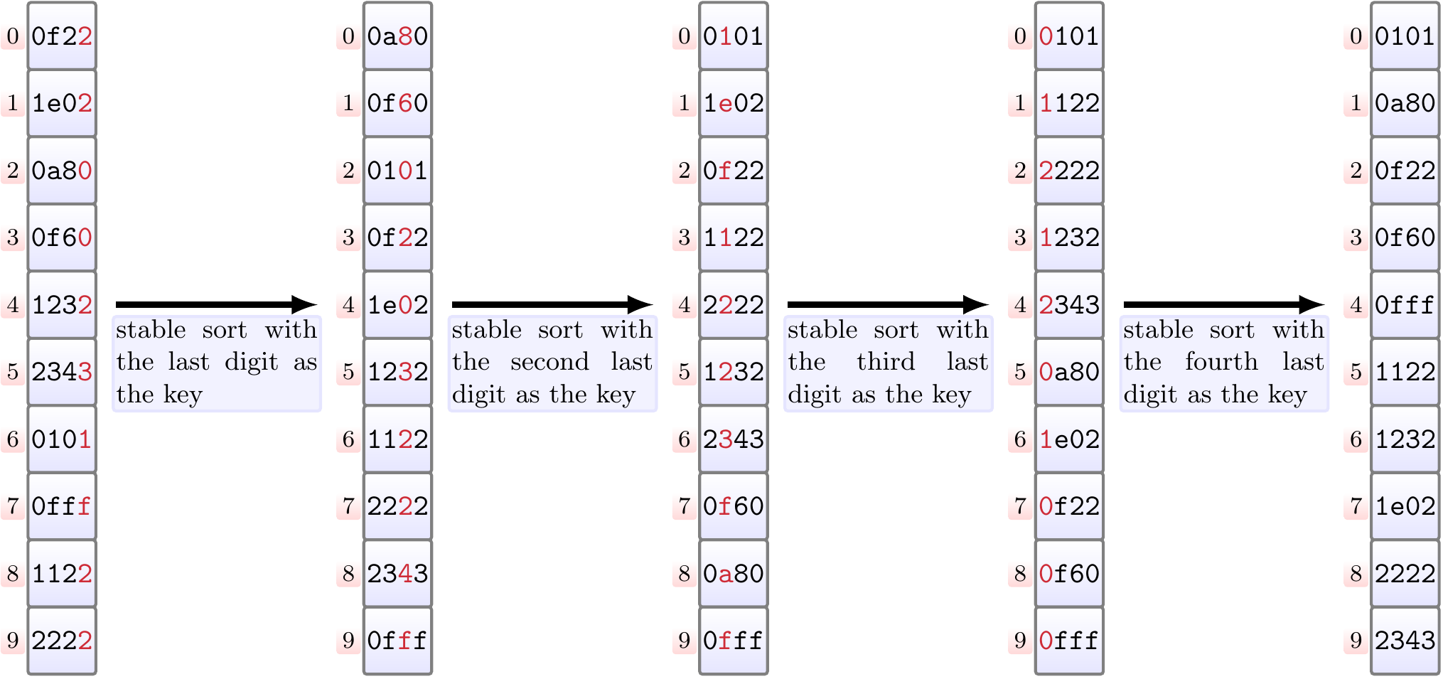
Example

Sorting 16-bit unsigned (hexadecimal) numbers with least-significant-digit-first radix sort by interpreting them as sequences of four 4-bit digits.

_images/radix-1.png

Properties:

  • ​ Stable.

  • ​ Needs \( \Theta(k+n) \) extra memory.

  • ​ Works in time \( \BigOh((k + n)d) \).

Implementation and experimental evaluation are left as a programming exercise.

Note that radix sort is used for sorting integers in the CUDA GPU Thrust library, see

  1. Satish, M. Harris and M. Garland: Designing Efficient Sorting Algorithms for Manycore GPUs, Proc. IEEE IDPDS 2009 (access via Aalto lib)