Priority queues with binary heaps¶

A binary heap is a tree data structure commonly used for

implementing priority queues, and
sorting (heapsort).

Abstractly, a priority queue is a container data structure that allows

inserting an element with some priority key,
finding an element with the largest key, and
removing an element with the largest key.

Equivalently, some implementations use the smallest priority instead of the largest. Note that multiple elements can have the same priority key. Thus an abstract data type for priority queues could have an API with:

\( \PQInsert{x} \) for inserting the element \( x \) with the key \( \TKeyOf{x} \).
\( \PQMax \) for getting an element with the largest key.
\( \PQRemove \) for removing an element with the largest key.
\( \PQIncrease{x}{v} \) for increasing the key of \( x \) to \( v \).
\( \PQDecrease{x}{v} \) for decreasing the key of \( x \) to \( v \).

Priority queus can be used, e.g., for

prioritizing network traffic based on the type or previous usage,
ordering pending orders according to the customer type,
building an event simulator, where events must be simulated in an order of the associated start times, and
selecting the best next option in other algorithms (Dijkstra’s algorithm later in this course etc).

Note that the elements are inserted and removed from the queue in an online fashion all the time. To implement priority queues, one could use resizable arrays and then apply an \( \Oh{n\Lg{n}} \) time sorting algorithm before each \( \PQMax \) and \( \PQRemove \) operation. But we can in fact do much better, so that each insert and remove takes \( \Oh{\Lg{n}} \) time if we currently have \( n \) elements in the queue.

Binary heaps and the heap property¶

A binary heap is a nearly-complete binary tree such that

all levels are full, except possibly the last one that is filled from left to right up to some point,
the nodes are associated with some elements having comparable keys (e.g., integers), and
the nodes satisfy a heap property:
- the key of each node is at least as large as that of any of its children (in which case the binary heap is a max-heap), or
- the key of each node is at least as small as that of any of its children (in which case the binary heap is a min-heap).

As a direct consequence, we have the following:

A binary heap with \( n \) nodes has height \( \Floor{\Lg n} \).
In a non-empty max-heap, an element with the largest key is in the root node.
In a non-empty min-heap, an element with the smallest key is in the root node.

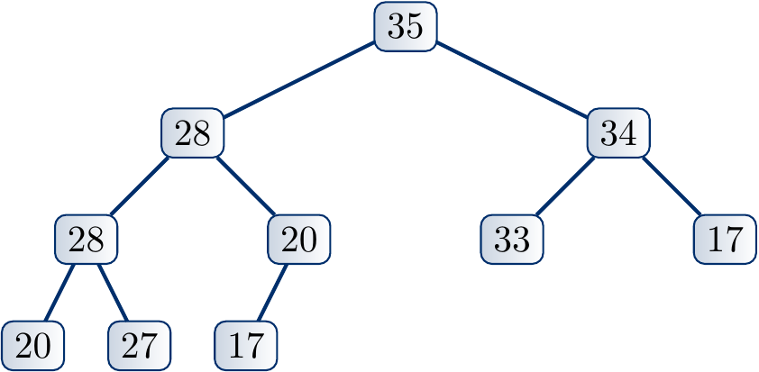
Example

Three nearly-complete binary trees, the keys of the elements associated with the nodes are shown inside the nodes.

The tree below is a max-heap.
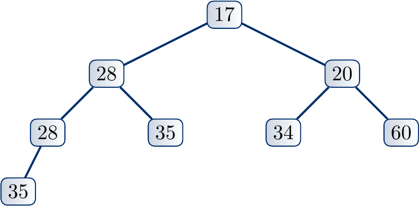
The tree below is a min-heap.
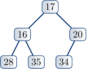
The tree below is neither a max-heap nor a min-heap.

Representing binary heaps¶

One does not usually represent binary heaps as node objects with pointers to children etc. Instead, as binary heaps are nearly-complete binary trees, they can be represented very compactly with (resizable) arrays. The idea is as follows:

A binary heap with \( n \) nodes is represented with a (resizable) array \( a \) of \( n \) elements.
The nodes are numbered from \( 0 \) to \( n-1 \) level-wise, left to right.
The element of the node \( i \) is stored in \( a[i] \)
The left child of the \( i \):th node is the node \( 2i+1 \). If \( 2i+1 \ge n \), then the \( i \):th node does not have a left child.
The right child of the \( i \):th node is the node \( 2i+2 \). If \( 2i+2 \ge n \), then the \( i \):th node does not have a right child
The parent of a non-root node \( i \) is the node \( \Parent{i} = \lfloor\frac{i-1}{2}\rfloor \).

Example

The figure below shows a max-heap (i) as a tree with the node numbers shown besides the nodes, and (ii) as an array.

Similarly, the figure below shows the tree and array representations for a min-heap.

Binary heap operations¶

In the following, we will only consider max-heaps — min-heaps can be handled in a similar, dual way. In the binary heap operations, such as inserting an element, we

start with a valid max-heap,
make a small modification, such as inserting an element at the end of the array, and
if the max-heap property is violated after the previous step, restore the max-heap property by a series of transformations.

The `upheap` and `increase-key` operations¶

The purpose of the upheap helper operation is to fix the max-heap property when we have increased the key of some element in the binary heap. The operation is also called swim and shift-up in some texts, and Heap-Increase-Key in the Introduction to Algorithms, 3rd ed. (online via Aalto lib) book. The increase-key operation then only increases the key of the element and calls upheap on that element.

Suppose that we increase the key of the node \( i \). The max-heap property can now be violated if the key becomes larger than that of the parent node \( \Parent{i} \). If this is the case, we swap the elements in the nodes \( i \) and \( \Parent{i} \). The max-heap property now holds in the sub-tree rooted at \( i \) as key of \( \Parent{i} \) was larger than that of \( i \) before the increase. But the max-heap property may now be violed if the key of the node \( \Parent{i} \) is larger than that of its parent. If this is the case, we (recursively) repeat the process at the parent node until the max-heap property is preserved in the whole tree.

At each step, a constant amount of steps is taken. The process repeats at most \( \Lg n \) times as it must stop when the root node is reached.

Example

The following steps illustrate the process of increasing the key of a node and applying upheap to restore the max-heap property

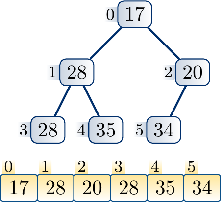
The max-heap in the beginning.
The tree after increasing the key of the node \( 4 \). The max-heap propery does not hold anymore.
upheap swaps the elements in the nodes \( 1 \) and \( 4 \).
upheap swaps the elements in the nodes \( 0 \) and \( 1 \). The max-heap property holds again.

The `downheap` and `decrease-key` operations¶

The purpose of the downheap helper operation is to fix the max-heap property after we have decreased the key of some element in the binary heap. It is also called sink and shift-down in some texts, and Max-Heapify in the Introduction to Algorithms, 3rd ed. (online via Aalto lib) book. The decrease-key operation then only decreases the key of the element and calls downheap on that element.

Suppose that we decrease the key of the node \( i \). The max-heap property becomes violated if the new key is smaller than that of any of its children. In such a case, we swap the elements of \( i \) and the child \( j \) with the larger key. After this, the key of \( i \) is now at least as large as the key of the other child. Furthermore, the key of \( i \) is smaller or equal to that of \( \Parent{i} \) because the original key of \( i \) was at least as large as that of \( j \). The max-heap property may now be violated if the new smaller key of \( j \) is smaller than that of any of its children. If this is the case, we (recursively) repeat the process from the node \( j \) until the max-heap property is preserved.

At each step, a constant amount of steps is taken. The process repeats at most \( \Lg n \) times as it must stop when a leaf node is reached.

Example

Decreasing the key of a node and applying down-heap to restore the max-heap property.

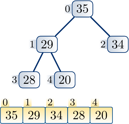
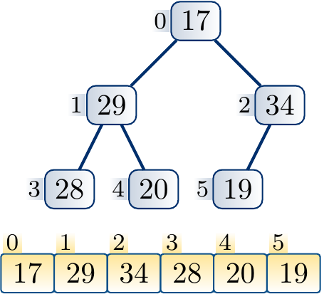
The max-heap in the beginning.
The tree after decreasing the key of the node \( 0 \). The max-heap propery does not hold anymore.
downheap swaps the elements in the nodes \( 0 \) and \( 2 \).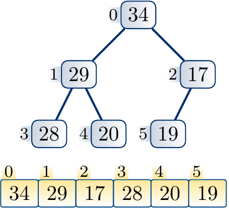
downheap swaps the elements in the nodes \( 2 \) and \( 5 \). The max-heap property holds again.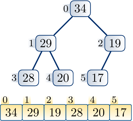

The `insert` operation¶

By using the upheap operation as a sub-routine, inserting a new element in a max-heap is easy:

Increase the size of the array by one and add the new element in the new node at the end of the array.
Apply upheap to the new node so that the max-heap property is restored.

Example: Applying the insert operation

The max-heap in the beginning:
Insert an element with the key \( 42 \) in the max-heap by adding it at the end of the resizable array. The max-heap property is now violated.
Apply upheap.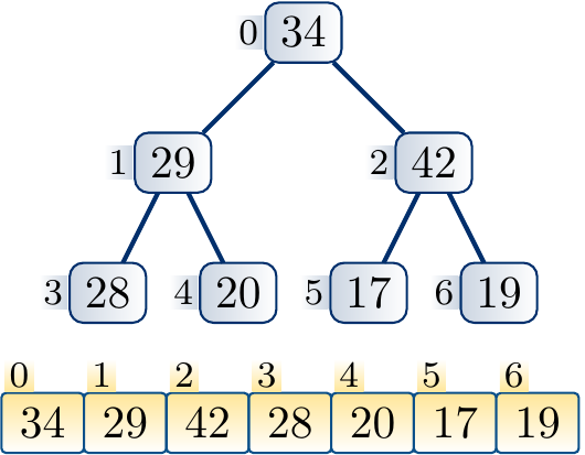
Apply upheap. The max-heap property holds again.

The `max` and `remove-max` operations¶

Implementing the max operation (getting an element with the largest key) is easy in max-heaps as the first element in the array has the largest key.

The remove-max operation that removes the first element in the array with the largest key can be implemented by using the downheap operation as a sub-routine:

Move the last node in the array to be the first node, effectively removing the element in the first index of the array. The key of this element is at most as large as that of the removed element.
Decrease the size of the resizable array by one.
Apply the downheap operation to the first node so that the max-heap property is restored.

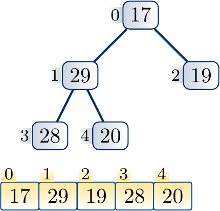
Example: Applying the remove-max operation

The max-heap in the beginning:
Remove the first element by moving the last element in its place. The size of the array is reduced by one. The max-heap propery is now violated.
Apply downheap.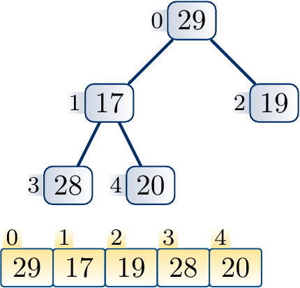
Apply downheap. The max-heap property holds again.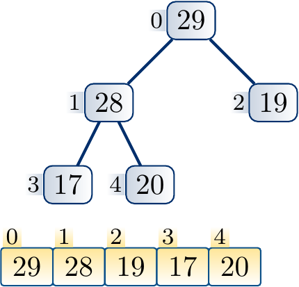

Implementations in some libraries¶

In Scala, the PriorityQueue class uses max-heaps.

Inserting elements and removing one with the largest key in \( \Oh{\Lg{n}} \) time.
Searching and removing an arbitrary element as well as many other methods in \( \Oh{n} \) time.
WARNING: do not use the max method to get the element with the maximum key, it is a linear time operation. Use the head method instead.

Example: constructing and using a priority queue of (string,integer) pairs with the integer field being the priority key.

scala> import collection.mutable.PriorityQueue
scala> val q = PriorityQueue[(String,Int)]()(_._2 compare _._2)
q: scala.collection.mutable.PriorityQueue[(String, Int)] = PriorityQueue()

scala> for((s,i) <- List("x","z","a","e","k") zip List(1,2,3,4,5)) q.enqueue((s,i))

scala> q
res1: ....PriorityQueue[(String, Int)] = PriorityQueue((k,5), (e,4), (z,2), (x,1), (a,3))

scala> while(q.nonEmpty) { println(q.head); q.dequeue }
(k,5)
(e,4)
(a,3)
(z,2)
(x,1)

Example: constructing and using a priority queue of (string,integer) pairs with the string field being the priority key. Observe that flipping the value of the comparison operator in the ordering argument of the priority queue constructor makes the queue to return the elements with the “smallest” strings first.

scala> import collection.mutable.PriorityQueue
scala> val q = PriorityQueue[(String,Int)]()((e1,e2) => -(e1._1 compare e2._1))
q: scala.collection.mutable.PriorityQueue[(String, Int)] = PriorityQueue()

scala> for((s,i) <- List("x","z","a","e","k") zip List(1,2,3,4,5)) q.enqueue((s,i))

scala> q
res1: ....PriorityQueue[(String, Int)] = PriorityQueue((a,3), (e,4), (x,1), (z,2), (k,5))

scala> while(q.nonEmpty) { println(q.head); q.dequeue }
(a,3)
(e,4)
(k,5)
(x,1)
(z,2)

In Java, the class java.util.PriorityQueue implements min-heaps.
- Inserting elements and removing one with the smallest key in \( \Oh{\Lg{n}} \) time.
- Searching and removing an arbitrary element in \( \Oh{n} \) time.
In the C++ standard library, the priority_queue class uses max-heaps.
- Inserting elements and removing one with the largest key in \( \Oh{\Lg{n}} \) time.
- No methods for searching arbitrary elements etc.

Interestingly, none of the above implement the increase-key or decrease-key operations.

Extra: Heapsort¶

This material is not included in the exam area of the course.

In addition to priority queues, binary heaps allow a natural idea for sorting: for the \( n \) elements to be sorted, insert them one by one in a min-heap and, after that, get and remove the minimum element of the queue \( n \) times. In this straightforward scenario, both phases (insertion and removal of all elements) can be done in \( \Oh{n \Lg n} \) time. However, we can do even better: (i) we can use the original array as a max-heap, (ii) perform the heap construction phase in linear time, and (iii) do the removal phase in the same array so that the result is a sorted array. We explain this heapsort algorithm below.

Suppose that we have a mutable array of \( n \) elements to be sorted. Consider the array as a representation of a binary heap (recall Section Representing binary heaps). Most likely, the binary heap is not a max-heap in the beginning but we can modify it, in linear time, so that the max-heap property holds. The procedure is as follows: from the second last level to the first level of the tree, apply downheap to all the nodes in the level.

Example: Phase 1 of the heapsort algorithm

The animation below illustrates the first phase of the heapsort algorithm: linear-time max-heap construction in the original array memory.

Let’s analyze the worst-case running time of the max-heap construction operation. Suppose that the tree has \( k \) levels, meaning that its height is \( k-1 \). The number \( n \) of nodes in it is thus \( 2^{k-1} \le n \le 2^k-1 \). The second-last level \( k-1-1 \) has at most \( 2^{k-1-1} \) nodes in it and each downheap operation does at most \( 1 \) swaps (the running time of a downheap operation is proportional to the number of swaps it makes). Similarly, the level \( k-1-i \) for an \( i \in [1 .. k-1] \) has at most \( 2^{k-1-i} \) nodes in it and each downheap operation does at most \( i \) swaps. Thus the max-heap construction makes at most \( \sum_{i=1}^{k-1} i 2^{k-1-i} = 2^{k-1} \sum_{i=1}^{k-1} \frac{i}{2^i} \) swaps. As \( \sum_{i=1}^{k} \frac{i}{2^i} < 2 \) for all \( k \in \mathbb{N} \) and \( 2^k = 2 \times 2^{k-1} \le 2 n \), we have \( \sum_{i=1}^{k-1} i 2^{k-1-i} \le 2^{k-1} 2 = 2^k \le 2 n \). Thus the running time of the max-heap construction is \( \Oh{n} \).

The phase two removes the elements from the max-heap one-by-one and inserts them in the correct place in the final sorted array, again using only the original array memory. This is done as follows. Initially all the \( n \) first elements are considered to represent a max-heap. The largest element is in the root. Then repeat the following until the heap contains only one element:

Swap the root with the last element in the array representing the heap.
After this, consider only the \( n-1 \) first elements to represent a max-heap.
Under the constraint, fix the max-heap property by applying downheap to the root.

Example: Phase 2 of the heapsort algorithm

The animation below shows the second phase of the heapsort algorithm: removing the maximum elements one-by.one and fixing the max-heap property in between. The same array memory is used to store the final sorted array.

Properties of heapsort:

Guaranteed worst-case running time is \( \Oh{n \Lg n} \).
Best-case running-time is \( \Oh{n} \): on arrays in which all the elements are the same, the downheap operations do not perform any swaps and the second phase of the algorithm also works in linear time.
Requires a constant amount of extra memory: only indices and two elements outside the array, no recursive function calls required.
Good for embedded systems with a limited amount of memory?

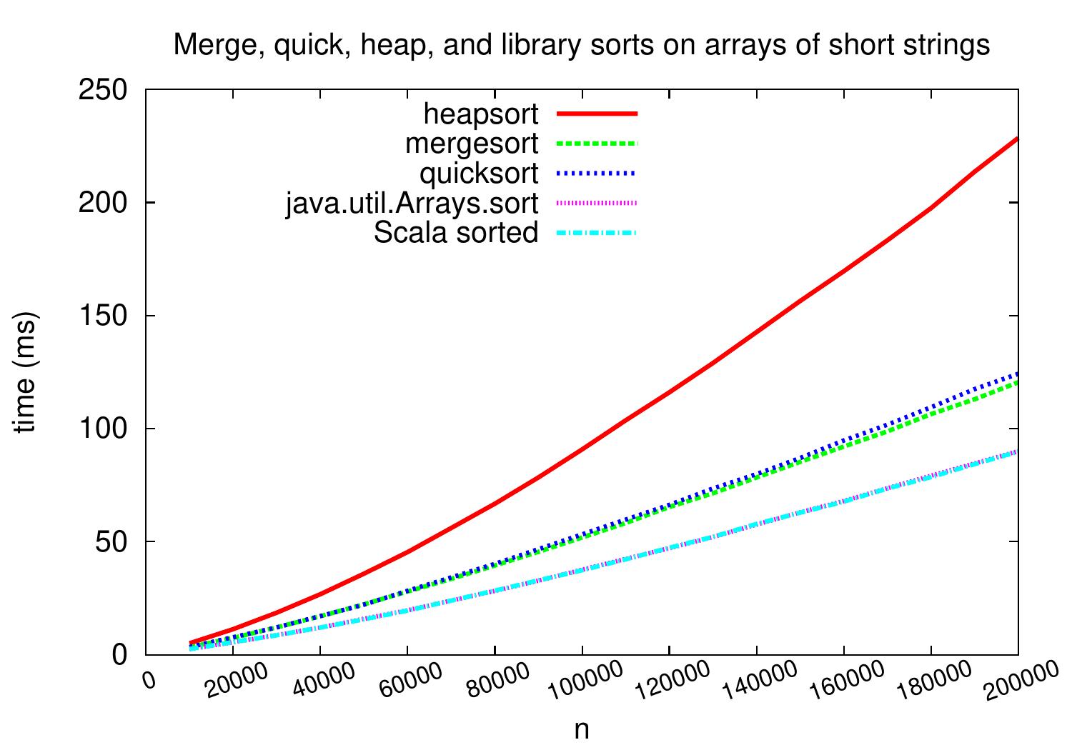
Experimental evaluation¶

The Scala code below gives an implementation of heapsort for arrays of integers, generalization to arbitrary comparable types is straightforward.

def heapsortInt(a: Array[Int]) {
  /*
   * The parent index of the node at index i.
   * Should not be called for the root node 0.
   */
  def parent(i: Int): Int = (i-1) / 2
  // The left child index of the node at the index i.
  def leftChild(i: Int): Int = 2*i+1
  // The right child index of the node at the index i.
  def rightChild(i: Int): Int = 2*i+2
  
  // Swap the lements at indices i and j.
  def swap(i: Int, j: Int) { val t = a(i); a(i) = a(j); a(j) = t }
  
  // Push the node at index "start" downwards
  // in the heap represented by the sub-array a[0..end].
  def downHeap(start: Int, end: Int) {
    var node = start
    while(leftChild(node) <= end) {
      var child = leftChild(node)
      var dest = node
      if(a(dest) < a(child))
        dest = child
      if(child+1 <= end && a(dest) < a(child+1))
        dest = child + 1
      if(dest == node) return
      swap(node, dest)
      node = dest 
    }
  }

  val n = a.length
  if(n <= 1) return
  
  // Build the initial heap
  var index = parent(n-1)
  while(index >= 0)  {
    downHeap(index, n-1)
    index -= 1
  }

  // Move the current largest element to the correct position
  // in the final result, apply downheap to the new root element.
  var end = n - 1
  while(end > 0) {
    // a(0) is the heap root, ie. the largest element in the current heap.
    // Move it to the correct position a(end) in the final result.
    swap(0, end)
    // Decrease the heap size by one
    end -= 1
    // Push the new root element down the heap
    downHeap(0, end)
  }
}

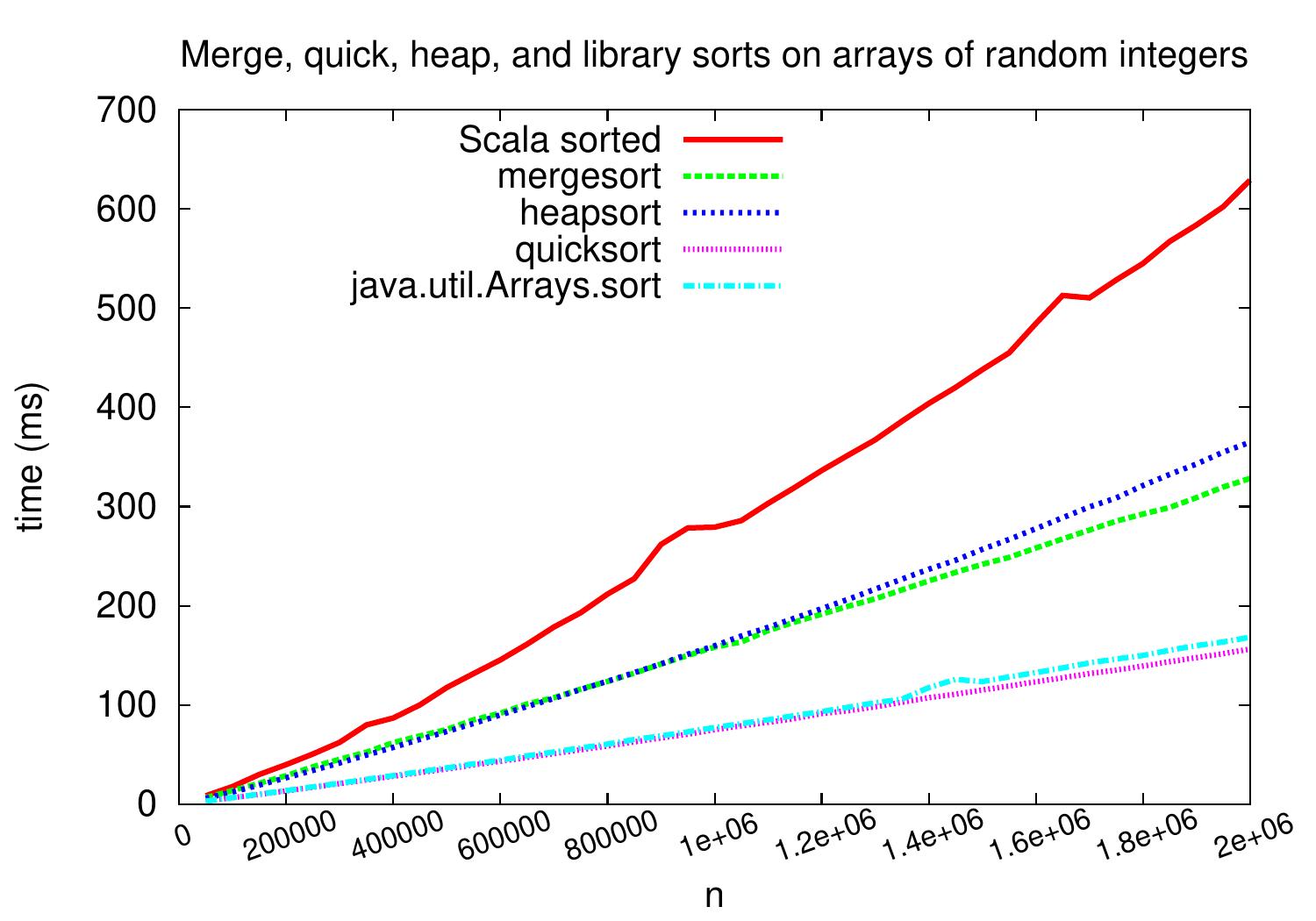
As we the next plot shows, on arrays of random integers the behavior of the heapsort implementation above is quite similar to that of Mergesort.

_images/benchmark-merge-quick-heap-library-ints-large.jpg

However, as shown in the figure below, heapsort is not that competitive on sorting arrays of strings.

_images/benchmark-merge-quick-heap-library-strings.jpg

Priority queues with binary heaps¶

Binary heaps and the heap property¶

Representing binary heaps¶

Binary heap operations¶

The upheap and increase-key operations¶

The downheap and decrease-key operations¶

The insert operation¶

The max and remove-max operations¶

Implementations in some libraries¶

Extra: Heapsort¶

Experimental evaluation¶

The `upheap` and `increase-key` operations¶

The `downheap` and `decrease-key` operations¶

The `insert` operation¶

The `max` and `remove-max` operations¶