Disjoint-sets with the union-find data structure¶

Another example of using trees as a data structure is representing disjoint sets. Such a disjoint sets data structure, or a union-find data structure, maintains a partitioning of a finite set \( S \) of elements into mutually disjoint subsets \( S_1,…,S_k \), meaning that

\( S_1 \cup … \cup S_k = S \) and
\( S_i \cap S_j = \emptyset \) for all \( 1 \le i < j \le k \).

In the beginning, each element \( a \) is in its own singleton set \( \Set{a} \). Given two elements \( x \) and \( y \), one can merge the sets \( S_x \) and \( S_y \) holding \( x \) and \( y \) into their union \( S_x \cup S_y \). A representative element is defined for each set and, for each element in the set, one can find this representative. Therefore, one can check whether two elements are in the same set by testing whether their representative elements are the same.

The abstract data type¶

The abstract data type for disjoint sets has the following methods:

\( \UFMS{x} \) introduces a new element \( x \) and puts it in its own singleton set \( \Set{x} \).
\( \UFFS{x} \) finds the current representative of the set that contains \( x \). Two elements \( x \) and \( y \) are in the same set if and only if their representatives are the same, i.e. when \( \UFFS{x} = \UFFS{y} \).
\( \UFUnion{x}{y} \) merges the sets of \( x \) and \( y \) to one set. This may change the representative of the elements in the resulting set.

Example: Testing whether an undirected graph is connected

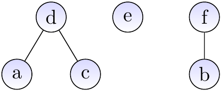
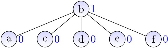
Consider the graph below.

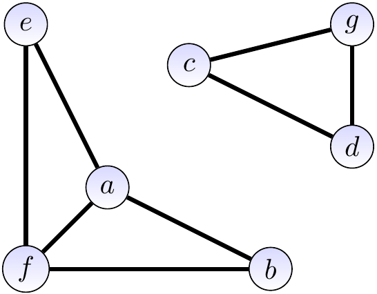
Let’s use a disjoint sets data structure to find out whether the graph is connected.

Initialize the disjoint-sets data structure by calling \( \UFMS{x} \) for each \( x \in \Set{a,b,c,d,e,f,g} \).

The disjoint sets are now \( \Set{a},\Set{b},\Set{c},\Set{d},\Set{e},\Set{f},\Set{g} \).
Next call \( \UFUnion{x}{y} \) for each edge \( \Set{x,y} \) in the graph.

After each call, two vertices \( x’ \) and \( y’ \) are in the same set if it is possible to reach \( x’ \) and \( y’ \) from each other by using only the edges considered so far.

For instance, after calling \( \UFUnion{a}{b} \) and \( \UFUnion{a}{e} \) because of the edges \( \Set{a,b} \) and \( \Set{a,e} \), the disjoint-sets are \( \Set{a,b,e},\Set{c},\Set{d},\Set{f},\Set{g} \).
At the end, the sets are \( \Set{a,b,e,f} \) and \( \Set{c,d,g} \).

As there is more than one set, the graph is not connected.

Two vertices \( x \) and \( y \) belong to the same connected component of the graph if \( \UFFS{x} = \UFFS{y} \).

The data structure and operations on it¶

Forests of rooted trees provide a simple way to represent disjoint sets. The idea is that each set is represented as a tree, the nodes in a tree containing the elements in the set. The root of the tree is the representative element of the set represented by that tree.

As the algorithms for the operations will only traverse the trees upwards, from nodes towards the root, we only need the parent reference for each node.

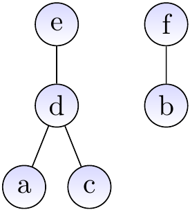
Example

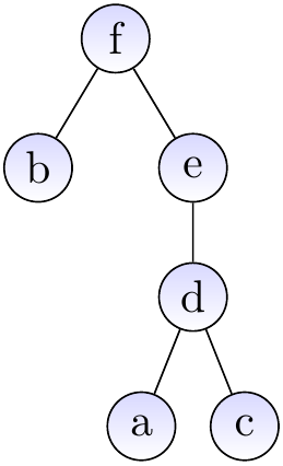
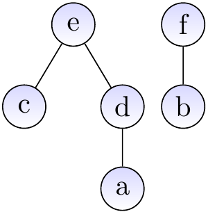
Suppose that we have introduced the elements \( a,b,…,f \) with \( \UFMS{} \) and then made unions so that the current sets are \( \Set{a,c,d,e} \) and \( \Set{b,f} \). The graph below shows one possible representation for the current situation. The representatives of the two sets are \( e \) and \( f \), respectively.

The `make-set` operation¶

Introducing a new element in the set data structure is easy: just introduce a new node that has no parent and is not a parent of any other node. As pseudocode:

// Insert the element \( x \) as a singleton set if not already in any set
\( \UFMS{x} \):
  if \( x \) is not yet in any set:
    insert \( x \) in some data structure recording the elements in the sets
    \( \UFParent{x} \Asgn \UFNil \)  // as a field or with a map
 

As mentioned earlier, we’ll only traverse the trees upwards and thus child references are not needed. For recording which elements appear in any of the sets (line 2 above) and associating elements to parents etc, one can use some standard map data structure (Scala’s HashMap or TreeMap, for instance) whose implementations are discussed in the next rounds of the course.

The `find-set` operation¶

To find the representative element for an element \( x \), we just

find the node of \( x \), and
traverse the parent pointers upwards to the root of the tree. The element at the root of the tree is the (current) representative of \( x \).

As pseudocode:

// Find the representative of the set containing \( x \)
\( \UFFS{x} \):
  raise an error if \( x \) is not in any set
  while \( \UFParent{x} \neq \UFNil \):
    \( x \Asgn \UFParent{x} \)
  return \( x \)
 

The `union` operation¶

Merging the sets of two elements to their union is quite easy as well:

First, find the roots of the trees containing the two elements.
If the roots are not the same, meaning that the elements are not yet in the same set, make the other tree to be a subtree of the another by making the parent pointer of its root to point to the root of the another tree.

As pseudocode

\( \UFUnion{x}{y} \):
  Check that \( y \) and \( y \) are in some set
  \( x' \Asgn \UFFS{x} \) // Find the root of the tree with \( x \)
  \( y' \Asgn \UFFS{y} \) // Find the root of the tree with \( y \)
  if \( x' \neq y' \): // Not yet in the same set?
    \( \UFParent{x'} = y' \) // Merge the trees by making \( x' \) a subtree of \( y' \)
 

Example: Inserting elements and making unions

First, call \( \UFMS{} \) for the elements \( a,…,f \). The forests are as follows.
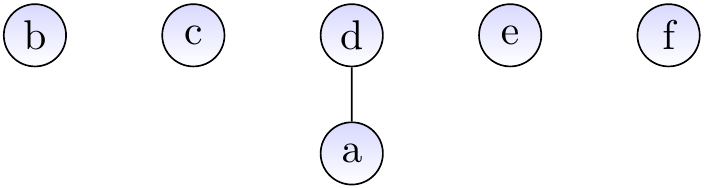
After calling \( \UFUnion{a}{d} \):
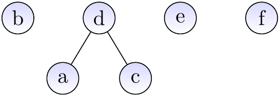
After calling \( \UFUnion{c}{a} \):
After calling \( \UFUnion{b}{f} \):
After calling \( \UFUnion{c}{e} \):
After calling \( \UFUnion{d}{b} \):

As one may expect, the basic versions of the operations given above do not guarantee the desired efficiency. In the worst case, the trees degenerate to “linear” trees that resemble linked lists and the find and union operations take linear time.

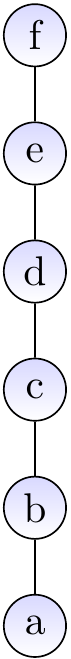
Example: Worst-case behaviour

Consider the following initial situation.

The result of applying \( \UFUnion{a}{b} \), \( \UFUnion{a}{c} \), \( \UFUnion{a}{d} \), \( \UFUnion{a}{e} \), and \( \UFUnion{a}{f} \) is the “linear” tree shown below.

Balancing with ranks¶

The problem with the tree in the previous example is that it is not “balanced”. If we can force the trees to be (at least roughly) balanced trees so that non-leaves have at least two children and the subtrees rooted at the children are roughly of the same size, a tree with \( n \) elements would have height \( \Oh{\Lg{n}} \) and the find-set and union operations would run in logarithmic time. Fortunately, there is a relatively easy way to do this:

Associate each node with a rank which is the height of the subtree rooted at the node,
When making an union, make the tree with smaller rank to be a child of the other one (if the ranks are the same, choose arbitrarily).

The updated pseudocode for the make-set operation is

// Insert the element \( x \) as a singleton set if not already in any set
\( \UFMS{x} \):
  if \( x \) is not yet in any set:
    insert \( x \) in some data structure recording the elements in the sets
    \( \UFParent{x} \Asgn \UFNil \)  // as a field or with a map
    \( \UFRank{x} \Asgn 0 \)       // as a field or with a map
 

and for the union operation:

\( \UFUnion{x}{y} \):
  Check that \( y \) and \( y \) are in some set
  \( x' \Asgn \UFFS{x} \) // Find the root of the tree with \( x \)
  \( y' \Asgn \UFFS{y} \) // Find the root of the tree with \( y \)
  if \( x' \neq y' \): // Not yet in the same set?
    if \( \UFRank{x'} > \UFRank{y'} \): // Subtree at \( x' \) has more height?
      \( \UFParent{y'} \Asgn x' \) // Merge the trees by making \( y' \) a subtree of \( x' \)
    else:
      \( \UFParent{x'} \Asgn y' \) // Merge the trees by making \( x' \) a subtree of \( y' \)
      if \( \UFRank{x'} = \UFRank{y'} \):
        \( \UFRank{y'} \Asgn \UFRank{y'}+1 \)
 

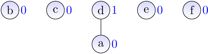
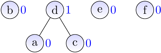
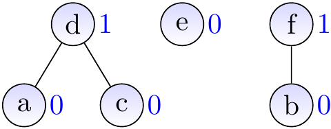
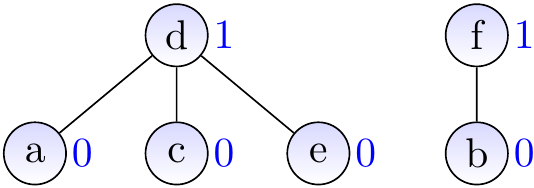
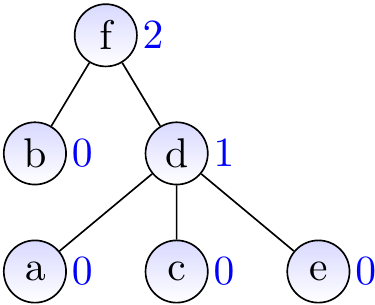
Example

Replay of our earlier example but now with ranks (shown besides the nodes):

In the beginning.
After calling \( \UFUnion{a}{d} \)
After calling \( \UFUnion{c}{a} \)
After calling \( \UFUnion{b}{f} \)
After calling \( \UFUnion{c}{e} \)
After calling \( \UFUnion{d}{b} \)

Example

Let’s replay of our earlier worst-case example but now with ranks. The result of applying \( \UFUnion{a}{b} \), \( \UFUnion{a}{c} \), \( \UFUnion{a}{d} \), \( \UFUnion{a}{e} \), and \( \UFUnion{a}{f} \) is no longer a linear tree but a very shallow one.

Theorem

With ranks, the height of each tree in the forest is at most \( \Floor{\Lg{\PParam}} \), where \( \PParam \) is the number of nodes in the tree.

Proof

By induction on the performed operations.

Induction base: the claim holds after \( 0 \) operations as there no trees in the forest.

Induction hypothesis: assume that the claim holds after \( m \) operations.

Induction step:

If we next perform a find operation, the trees do not change and thus the claim holds for \( m+1 \) operations.
If we insert a new element, we insert a new isolated node (a tree with \( 1 \) node and of height \( 0 = \Floor{\Lg 1} \)) and the other trees stay the same. As any other tree was of height \( \Floor{\Lg{\PParam}} \) or less by the induction hypothesis, the tree is of height \( \Floor{\Lg(\PParam+1)} \) or less after the operation.
If we make union operation on \( x \) and \( y \), we have two cases.
1. If the elements are in the same set, the trees stays unmodified.
2. If the elements are in different sets of sizes \( \PParam_x \) and \( \PParam_y \), then the heights of the corresponding trees are, by induction hypothesis, \( h_x \le \Floor{\Lg{\PParam_x}} \) and \( h_y \le \Floor{\Lg{\PParam_y}} \).
  - If \( h_x < h_y \), then the resulting tree has \( \PParam_x + \PParam_y \) nodes and height \( h_y \). As \( h_y \le \Floor{\Lg{\PParam_y}} \), \( h_y \le \Floor{\Lg(\PParam_x + \PParam_y)} \).
  - The case \( h_y < h_x \) is symmetric to the previous one.
  - If \( h_x = h_y \), then the resulting tree has \( \PParam’ = \PParam_x + \PParam_y \) nodes and height \( h’ = h_x + 1 = h_y + 1 \).
    
    If \( \PParam_x \le \PParam_y \), then \( \PParam’ \ge 2\PParam_x \) and \( \Floor{\Lg(\PParam’)} \ge \Floor{\Lg(2 \PParam_x)} = \Floor{\Lg(2) + \Lg \PParam_x} = 1+\Floor{\Lg \PParam_x} = h’ \).
    
    Similarly, if \( \PParam_x \ge \PParam_y \), then \( \PParam’ \ge 2\PParam_y \) and \( \Floor{\Lg(\PParam’)} \ge \Floor{\Lg(2 \PParam_y)} = \Floor{\Lg(2) + \Lg \PParam_y} = 1+\Floor{\Lg \PParam_y} = h’ \).

Therefore, the claim holds after \( m+1 \) operations and by the induction principle, the claim holds for all values \( m \).

Let \( n \) be the number of elements in the current disjoint sets. Assume that we can

find the node of each element in \( \Oh{\Lg{n}} \) time, and
access and modify the parent and rank values in constant time.

Under these assumptions and by using ranks, the make-set, find-set and union operations take \( \Oh{\Lg{n}} \) time.

Path compression¶

Path compression is another idea for making the trees even shallower. As it name implies, it compresses the paths from the nodes to the roots during the find-set operations. We perform a (recursive) search to find the root from a node, and after each recursive call update the parent of the current node to be the root. As pseudocode:

// Find the representative of the set containing \( x \)
\( \UFFS{x} \):
  raise an error if \( x \) is not in any set
  def \( \UFCompress{y} \):
    if \( \UFParent{y} = \UFNil \): // In the root?
      return \( y \)
    else
      \( r \Asgn \UFCompress{\UFParent{y}} \)
      \( \UFParent{y} \Asgn r \)
      return \( r \)
  return \( \UFCompress{x} \)
 

Observe that the find-set operation is also called during the union operation, and thus path compression may occur there as well.

Example

Assume that we have the disjoint-sets forest shown below.

When we call \( \UFFS{c} \), the forest is modified to illustrated below.

Theorem

With union-by-rank and path compression, making \( m \) disjoint-set operations on \( n \) elements takes \( \Oh{m \alpha(m)} \) time, where \( \alpha \) is a very slowly growing function with \( \alpha(m) \le 4 \) for all \( m \le 2^{2048} \).

Proof

See Section 21.4 in Introduction to Algorithms, 3rd ed. (online via Aalto lib). The proof is not required in the course.

Disjoint-sets with the union-find data structure¶

The abstract data type¶

The data structure and operations on it¶

The make-set operation¶

The find-set operation¶

The union operation¶

Balancing with ranks¶

Path compression¶

The `make-set` operation¶

The `find-set` operation¶

The `union` operation¶