Basic definitions
Trees are a special subclass of graphs (we’ll consider graphs and graph algorithms in more detail in Round 7: Graphs, part I and Round 8: Graphs, part II). Mathematically, an undirected graph is a pair \( \Tuple{\Verts,\Edges} \), where
\( \Verts \) is a (usually finite) set of vertices, also called nodes, and
\( \Edges \) is a set of edges between the vertices. Each edge in the set is a pair of the form \( \Set{u,v} \) such that \( u,v \in \Verts \) and \( u \neq v \). Thus self-loops, meaning edges between vertex and itself, are not allowed in undirected graphs under this definition.
Example
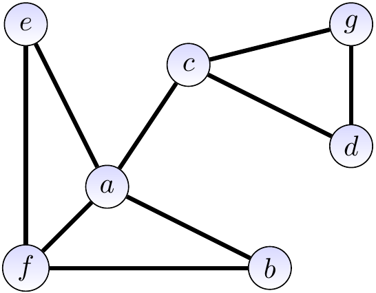
Consider the graph \( \Tuple{\Verts,\Edges} \) with
the vertices \( \Verts = \Set{a,b,c,d,e,f,g,h} \), and
the edges \( \Edges = \{\Set{a,b},\Set{a,c},\Set{a,e},\Set{a,f},\Set{b,f},\Set{e,f},\Set{c,d},\Set{c,g},\Set{d,g}\} \).
It is illustrated graphically below. The vertices drawn as circles and edges as lines between the vertices.
A path of length \( k \) from a vertex \( v_0 \) to a vertex \( v_k \) is a sequence \( \Path{v_0,v_1,…,v_k} \) of \( k+1 \) vertices such that \( \Set{v_{i-1},v_{i}} \in \Edges \) for each \( i \in [1 .. k] \). A vertex \( v \) is reachable from a vertex \( u \) if there is a path from \( u \) to \( v \). Note that each vertex is reachable from itself as there is a path of length \( 0 \) from the vertex to itself. A path is simple if all the vertices in it are distinct. The graph is connected if every vertex in it is reachable from all the other vertices.
Example
The graph shown below
has a (non-simple) path \( \Path{a,c,d,g,c,d} \) of length 5 from \( a \) to \( d \),
has a simple path \( \Path{a,c,d} \) of length 2 from \( a \) to \( d \), and
is connected but deleting the edge \( \Set{a,c} \) would make it disconnected
A cycle is a path \( \Path{v_0,v_1,…,v_k} \) with \( k \ge 3 \) and \( v_0 = v_k \). A cycle \( \Path{v_0,v_1,…,v_k} \) is simple if \( v_1,v_2,…,v_k \) are all distinct. A graph is acyclic if it does not have any simple cycles.
Example
The graph shown below is not acyclic as it contains, among some others, a simple cycle \( \Path{a,e,f,a} \).
On the other hand, the graph drawn below is acyclic.
Trees and forests
A free tree is a connected, acyclic, and undirected graph. We usually omit “free” and just speak of “trees”. An undirected graph that is acyclic but not necessarily connected is called a forest.
Example
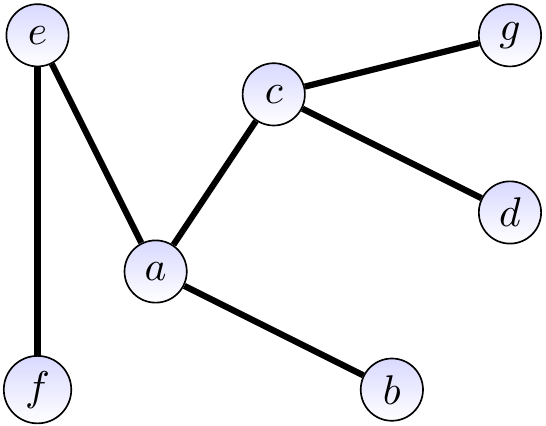
The graph below is a free tree.

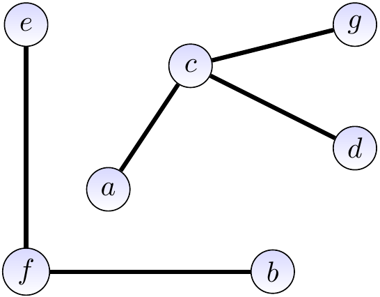
The graph below is a forest of two trees.
Theorem: B.2 in Introduction to Algorithms, 3rd ed. (online via Aalto lib)
If \( G = \Tuple{\Verts,\Edges} \) is an undirected graph, then the following statements are equivalent:
\( G \) is a free tree.
Any two vertices in \( G \) are connected by a single simple path.
\( G \) is connected but removing any edge from it makes it disconnected.
\( G \) is connected and \( \Card{\Edges} = \Card{\Verts}-1 \).
\( G \) is acyclic and \( \Card{\Edges} = \Card{\Verts}-1 \).
\( G \) is acyclic but adding any edge to it would make it to contain a cycle.
Rooted trees
A rooted tree is a free tree in which one vertex is a special one called the root of the tree.
Example
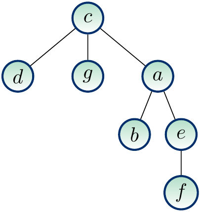
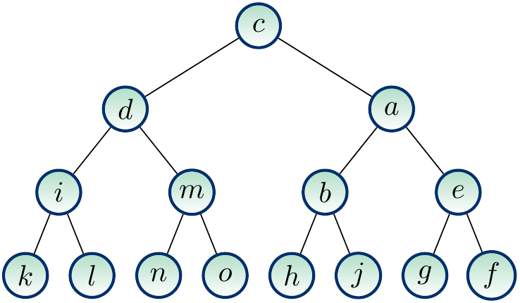
The figure below shows a rooted version of our earlier free tree when the root node is \( c \). When we draw rooted trees, the root is always drawn in the same place, usually at top.
Again, we speak only of “trees” instead of “rooted trees” when it is clear from the context that the trees are rooted. Take any rooted tree with the root node \( r \). We make the following definitions.
Any node \( y \) on the unique simple path from \( r \) to a node \( x \) is an ancestor of \( x \).
If \( y \) is an ancestor of \( x \), then \( x \) is a descendant of \( y \).
If \( y \) is an ancestor of \( x \) and \( x \neq y \), then \( y \) is a proper ancestor of \( x \) and \( x \) is a proper descendant of \( y \).
If \( y \) is a ancestor of \( x \) and \( \Set{y,x} \) is an edge, then \( y \) is the unique parent of \( x \) and \( x \) is a child of \( y \).
If two nodes have the same parent, they are siblings.
The root has no parent and a node with no children is a leaf.
The leaf nodes are also called external nodes and the non-leaf ones internal nodes.
Example
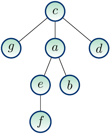
On the rooted tree shown below,
the ancestors of \( e \) are \( e \), \( a \) and \( c \),
the descendants of \( a \) are \( a \), \( b \), \( e \) and \( f \),
the parent of \( a \) is \( c \) and its children are \( b \) and \( e \), and
the leaves are \( d \), \( g \), \( b \) and \( f \).
The subtree rooted at a node \( x \) is the tree induced by the descendants of \( x \).
The length of the simple path from the root to a node \( x \) is the depth of \( x \).
A level consists of all nodes at the same depth.
The height of a node \( x \) is the length of the longest simple path from it to any leaf node.
The height of the tree is the height of its root node.
Example
On the rooted tree below,
the subtree rooted at \( a \) contains the nodes \( a \), \( b \), \( e \) and \( f \),
the depth of \( b \) is 2,
the nodes at the level 1 are \( d \), \( g \) and \( a \),
the height of \( a \) is 2, and
the height of the tree is 3.
An ordered tree is a rooted tree where the children of each node are ordered. That is, if a node has \( k \) children, then one of them is the first one, another is the second one and so on.
Example
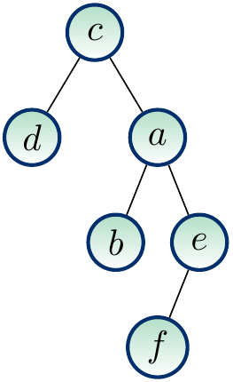
Consider the ordered tree shown below. The first child of \( c \) is \( d \), the second is \( g \) and the third is \( a \).
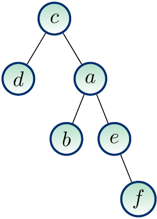
The tree shown below is different to that shown above when we consider the trees to be ordered. If they were considered unordered, then they would be the same.
Binary trees
Binary trees are a special class of ordered trees where each node
has at most two children, the left child and the right child, and
either of them or both can be missing.
This is different from 2-ary ordered trees (an ordered tree with maximum degree of at most 2) because if a node has one child, it makes a difference whether it is the left or the right child.
Example
The trees below are binary trees; naturally, the left child is drawn on the left of the parent, the right on the right. They are different binary trees but would be the same if they were considered only as ordered trees.
A binary tree is full if each node in it is either a leaf or an internal node with exactly two children. A binary tree is complete if it is full and all the leaves have the same depth. (Note: in some texts, the “complete” binary trees as defined above are called “perfect” binary trees.)
Example
The tree below is neither full nor complete.
The tree below is full but not complete.
The tree below is complete.
A complete binary tree of height \( h \) has
\( 2^h \) leaves, and
\( 2^h-1 \) internal nodes.
Exercise: prove the above claim by using induction on the height of the tree. As a direct consequence, a complete binary tree with \( n \) leaves has height \( \Lg{n} \).
Data structures for trees
There is no single universally best data structure for trees in general. This is because different tree types can be represented in different ways. Furthermore, different algorithms on trees need different information. For instance,
some need to traverse trees downwards and thus need to find the children of a node, but
some only need the parent information.
As a concrete example, in the section Priority queues with binary heaps, trees of certain type will be represented with arrays so that the child/parent information is not represented explicitly at all. Similarly, in the section Disjoint-sets with the union-find data structure only the parent information is attached to each node.
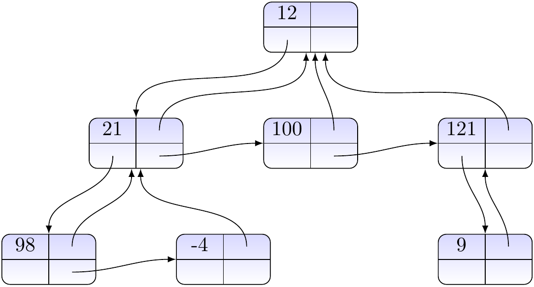
One generic way to represent binary trees is to store the nodes as objects so that each object has references to
the parent node (if the node is root, either \( \NULL \) or the node itself),
the left and right children (\( \NULL \) if missing), and
some key/value/etc as we usually use trees to store/reference other data.
Example
Let us use the graphical notation
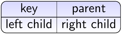
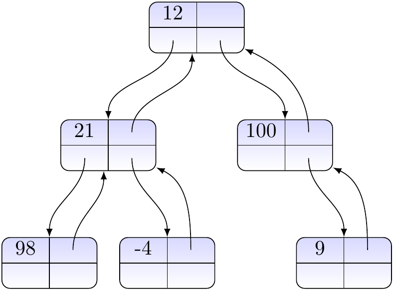
for the node objects. Consider the tree below. Here we are not interested in node names but show the keys/values associated to the nodes inside them.

The tree can be represented with the object diagram
As a second example, one way to represent trees in which nodes can have unbounded amount of children is to have each node reference to the first child and to the next sibling.
Example
Using the representation
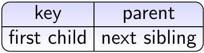
for nodes, the tree

is represented with the following objects:
In this representation, random access to \( i \)th child of a node with \( n \) children requires \( \Theta(n) \) time in the worst case but iterating over all children is easy.