Single-source shortest paths¶

In many applications we are interested in the shortest paths between two vertices. For instance, what is the shortest distance (or the fastest route if the weights are driving times) between two addresses in a road map? In edge-weighted graphs we speak of “shortest paths” but in fact mean paths with smallest cumulative weight, not paths with fewest number of vertices in them as in the case of graphs with no edge weights.

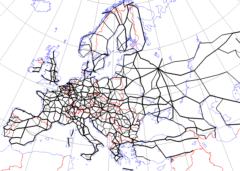
_images/International_E_Road_Network.png

(Figure: public domain, source)

The weight of a path $ p = \Path{v_0,v_1,…,v_k} $ is the sum of the weights of its edges: $ w(p) = \sum_{i=0}^{k-1}\Weight{v_i}{v_{i+1}} $. The shortest-path weight $ \SPDist{u}{v} $ between two vertices $ u $ and $ v $ is

the minimum of the weights of all paths from $ u $ to $ v $, or
$ \infty $ if there is no path from $ u $ to $ v $.

Example

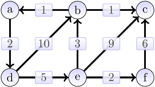
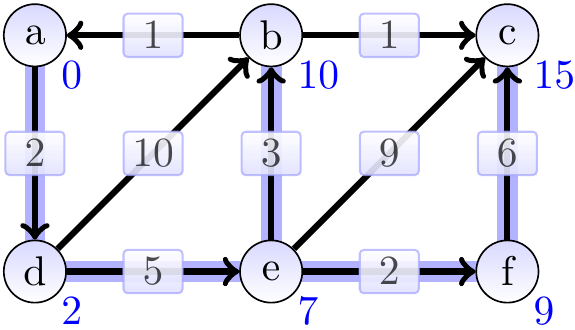
Consider the graph below. The shortest-path weight from $ a $ to $ c $ is 11 produced by the path $ \Path{a,d,e,b,c} $. On the other hand, $ \SPDist{f}{b} = \infty $ as there is no path from $ f $ to $ b $.

In this section, we consider the following single-source shortest paths problem asking for a shortest path from a source vertex to each other vertex.

Definition: Single-source shortest paths

Given a directed, edge-weighted graph and a source vertex $ s $ in it.

Find a shortest path from $ s $ to each vertex that is reachable from $ s $.

We could also consider a restricted variant of the problem:

Definition: Single-pair shortest path

Given a directed, edge-weighted graph and two vertices, $ u $ and $ v $, in it.

Find a shortest path from $ u $ to $ v $.

But the basic algorithms for the latter have the same worst-case asymptotic running time as the best algorithms for the first, so in the following we consider the more generic single-source shortest paths problem (see Further reading for references to some advanced algorithms). The presented algorithms differ in whether they can handle negative-weight edges and in the worst-case running time.

Observe that the shortest path have an “optimal substructure” property: sub-paths of shortest paths are shortest paths. That is, if $ \Path{v_0,v_1,…,v_i,…,v_k} $ is a shortest path from $ v_0 $ to $ v_k $, then

$ \Path{v_0,v_1,…,v_i} $ is a shortest path from $ v_0 $ to $ v_i $, and
$ \Path{v_i,…,v_k} $ is a shortest path from $ v_i $ to $ v_k $.

We have to pay special attention to negative edge weights when considering “shortest paths”, which are actually “paths with the smallest cumulative weight”. We say that a cycle $ p = \Path{v_0,…,v_k,v_0} $ is a negative-weight cycle (or simply a “negative cycle”) if $ w(p) < 0 $. If any path from a vertex $ u $ to $ v $ contains a negative cycle, then the shortest-path weight from $ u $ to $ v $ is not well-defined and we may write $ \SPDist{u}{v} = -\infty $.

Example

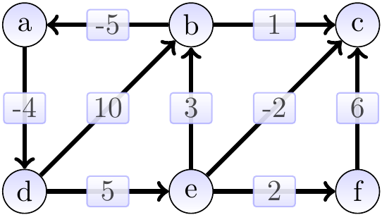
Consider the graph below. It has a negative-weight cycle $ \Path{a,d,e,b,a} $. Thus the shortest-path weight from $ a $ to $ f $ is not well-defined as one can first repeat the cycle arbitrarily many times and then take the path $ \Path{a,d,e,f} $.

Shortest-path weight estimates and relaxation¶

The algorithms given later maintain, for each vertex $ \Vtx $, a shortest-path weight estimate $ \SPEst{\Vtx} $. The estimate is

always an upper bound for the shortest-path weight: $ \SPEst{\Vtx} \ge \SPDist{\SPSrc}{\Vtx} $, and
at the end, if there are no negative cycles, equal to the shortest-path weight: $ \SPEst{\Vtx} = \SPDist{\SPSrc}{\Vtx} $.

In addition, the shortest paths form a shortest-paths tree rooted at the source vertex $ \SPSrc $ and the predecessor of a vertex $ \Vtx $ in this tree is saved in the attribute $ \SPPred{\Vtx} $. Initially,

the estimates are $ \infty $ for all the nodes except that for $ \SPSrc $ it is 0, and
all the predecessor attributes are $ \SPNil $.

Initialization as pseudo-code:

Initialize-single-source(\( G \), \( \SPSrc \)):
  for each vertex \( \Vtx \in \Verts \):
    \( \SPEst{\Vtx} = \infty \)
    \( \SPPred{\Vtx} = \SPNil \)
  \( \SPEst{\SPSrc} = 0 \)
 

If for some edge $ (u,v) $ it holds that $ \SPEst{u} + \Weight{u}{v} < \SPEst{v} $, we can think that the edge has “tension” and perform a relaxation step updating the estimate of $ v $ to $ \SPEst{v} = \SPEst{u} + \Weight{u}{v} $. The predecessor of $ v $ is set to $ u $ as the shortest known path from the source vertex to $ v $ now comes via the vertex $ u $. In pseudo-code:

Relax(\( u \), \( v \)):
  if \( \SPEst{u}+\Weight{u}{v} < \SPEst{v} \):
    \( \SPEst{v} = \SPEst{u}+\Weight{u}{v} \)
    \( \SPPred{v} = u \)
 

The relaxation step is the only place where the estimate is modified. The algorithms shown below differ in which order, and how many times, the estimates are relaxed. The relaxation preserves the upper bound property of the estimates:

If $ \SPEst{\Vtx} \ge \SPDist{\SPSrc}{\Vtx} $ holds for all vertices $ \Vtx $ before a relaxation step, the same also holds after the relaxation step.

Dijkstra’s algorithm¶

Dijkstra’s algorithm is a greedy algorithm for computing single-source shortest paths. It assumes that all the edge weights are non-negative. The high-level idea is as follows:

Initialize the estimate attributes as described above ($ 0 $ for the source vertex $ \SPSrc $ and $ \infty $ for the others).
In each of the at most $ \NofV $ iterations:
- Take a vertex $ u $ that has not yet been considered and that has the smallest known shortest-path weight estimate from the source vertex (which is in fact equal to the shortest-path weight at this point).
  
  The first iteration thus considers the source vertex.
- Consider each edge from the vertex and perform relaxation if possible. That is, update the estimate of the target vertex $ v $ if a shorter path from the source to $ v $ is obtained by a path via the vertex $ u $.

In pseudo-code:

Dijkstra(\( G = \Tuple{\Verts,\Edges,\Weights} \), \( \SPSrc \)):
  Initialize-single-source(\( G \), \( \SPSrc \))
  let \( S = \emptyset \)
  let \( Q = \Verts \)   // Min-priority queue with the distance attribute as the key
  while \( Q \neq \emptyset \):
    let \( u \) be a vertex with minimum \( \SPEst{u} \) in \( Q \)
    remove \( u \) from \( Q \)
    let \( S = S \cup \Set{u} \)
    for each vertex \( v \) with \( (u,v) \in \Edges \):
      Relax(\( u \), \( v \))
 

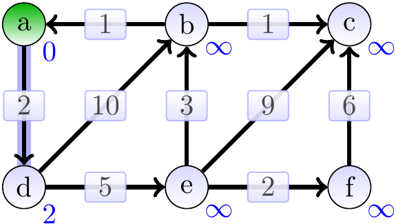
Example: Applying Dijkstra’s algorithm

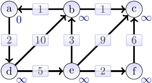
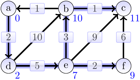
Consider the graph below, the annotations showing the estimate attributes in the beginning. The source vertex is $ a $.

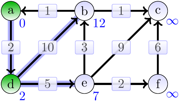
The graphs below show the estimates and the constructed shortest paths (the highlighted edges) after each loop iteration. The green vertices are the ones in the set $ S $ in the pseudo-code. First, we remove $ a $ from the min-priority queue and update the estimates of its neighbors.

Next, the vertex $ d $ has the smallest estimate (which in fact is the correct shortest-path weight from $ a $ to $ d $) and we dequeue it from the queue and update the estimates of its neighbors.

The vertex $ e $ is dequeued next. Observe that the estimate of $ b $ is improved from $ 12 $ to $ 10 $.

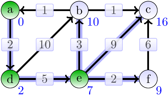
The vertex $ f $ is dequeued next.

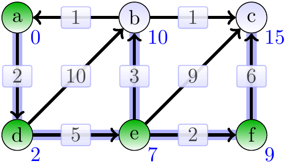
The vertex $ b $ is dequeued next.

Finally, the vertex $ c $ is dequeued.

Constructing the shortest path from $ a $ to $ c $ is now easy: just start from $ c $ and follow the predecessor edges back to $ a $.

A worst-case running time analysis of the algorithm, assuming that the priority queues are implemented with heaps (recall Section Priority queues with binary heaps):

Initialization phase takes $ \Oh{\NofV} $ time. Initializing the priority queue takes time $ \NofV \Lg{\NofV} $ when done in the straightforward way but could also be done in time $ \Oh{\NofV} $.
The while-loop executes at most $ \NofV $ times, once for each vertex $ u $.
- Taking the vertex $ u $ from the priority queue takes time $ \Oh{\Lg{\NofV}} $.
- Each edge from $ u $ is traversed once.
- Relaxation of the edge $ \Tuple{u,v} $ takes time $ \Oh{\Lg{\NofV}} $: when the estimate attribute is updated, the priority queue is updated as the estimate attribute is its key.

The total is thus $ \Oh{\NofV + \NofV \Lg{\NofV} + \NofV \Lg{\NofV} + \NofE\Lg{\NofV}} = \Oh{(\NofV + \NofE)\Lg{\NofV}} $. For graphs in which all the vertices are reachable from the source vertex this equals to $$\Oh{\NofE\Lg{\NofV}}$$ as $ \NofE \ge \NofV-1 $ in such a case.

Correctness can be argued by proving the following invariant:

Lemma

At the end of each iteration, if there is a path from the source vertex $ s $ to $ t $ and $ t \in S $, then $ \SPEst{t} = \SPDist{s}{t} $.

Proof

By induction on the size of the set $ S $:

Base case: when $ \Card{S} = 1 $, then $ S = \Set{s} $ and $ \SPEst{s} = \SPDist{s}{s} = 0 $ (relaxing a loop from $ s $ to itself cannot change $ \SPEst{s} $ from $ 0 $ as the edge weights are non-negative)
Induction hypothesis: assume that the invariant holds when $ \Card{S} = k $ for some $ k \ge 1 $
Induction step: let $ u $ be a vertex not in $ S $ having the smallest $ \SPEst{u} $ among such vertices.

If $ \SPEst{u} = \infty $, there is no edge from any vertex $ x \in S $ to any vertex $ y \notin S $ as all the outgoing edges from the vertices in $ S $ have been relaxed already. Thus $ \SPDist{s}{u} = \infty $ and the invariant holds after the $ k+1 $:th iteration when $ S \cup \Set{u} $.

Otherwise, $ \SPEst{u} \neq \infty $.

Now $ \SPPred{u} \in S $ and there is a path $ \Path{s,…,\SPPred{u},u} $ of weight $ d = \SPEst{u} = \SPDist{s}{\SPPred{u}} + \Weight{\SPPred{u}}{u} $ from $ s $ to $ u $ so that the second last vertex in the path is $ \SPPred{u} $. To see that this is a shortest path from $ s $ to $ u $, assume that $ \SPDist{s}{u} < d $ and a shortest is a path $ \Path{s,…,x,y,…u} $ with $ y $ being the first vertex in the path not in $ S $. As $ \Path{s,…,x,y,…u} $ is the shortest one and the edge weights are non-negative, $ \SPDist{s}{y} < d $ and $ \SPDist{s}{x} < d-\Weight{x}{y} $. As $ x \in S $, $ \SPEst{x} = \SPDist{s}{x} $ and the edge $ \Tuple{x,y} $ has been relaxed before, implying that $ \SPEst{y} = \SPDist{s}{y} < d $. But in such a case $ u $ would not be a vertex with the smallest $ \SPEst{u} $ among the vertices not in $ S $, a contradiction. Thus $ \SPEst{u} = \SPDist{s}{u} $ and $ \Path{s,…,\SPPred{u},u} $ is a shortest path from $ s $ to $ u $.

After inserting $ u $ to $ S $, relaxing an edge $ \Tuple{u,v} \in E $ for a $ v \in S $ does not change the value $ \SPEst{v} $ as $ \SPEst{v} = \SPDist{s}{v} $ already by the induction hypothesis.

Thus the invariant holds after the $ k+1 $:th iteration when $ S \cup \Set{u} $.

The next example illustrates why negative edges, even when there are no negative-weight cycles, can be a problem for Dijkstra’s algorithm.

Example: The problem with negative-weight edges

Consider the graph with a negative-weight edge shown below. As the animation shows, the edges from the vertex $ c $ are traversed only once when the vertex $ c $ is taken away from $ Q $. In the presence of the negative edges, the estimate at that point is not the shortest-path weight here and the estimates of the vertices reachable from $ c $ are not evaluated correctly.

The Bellman-Ford algorithm¶

The Bellman-Ford algorithm is also an algorithm for computing single-source shortest paths. The difference to Dijkstra’s algorithms is that negative edge weights are now allowed and the algorithm can detect whether the graph has a negative-weight cycle. The basic idea:

Relax all the edges $ \Card{\Verts}-1 $ times.
If relaxation is still possible, there is a negative-weight cycle.

Otherwise, the estimates are exact and give the shortest-path weights.

Thus the negative-weight problem of Dijkstra’s algorithm is cured by re-evaluating the estimates of the neighbor vertices whenever the estimate of the vertex is decreased. In pseudo-code:

Bellman-Ford(\( G \), \( \SPSrc \)):
  Initialize-single-source(\( G \), \( \SPSrc \))
  for \( i = 1 \) to \( \Card{\Verts}-1 \):
    for each edge \( (u, v) \in \Edges \):
      Relax(\( u \), \( v \))
  for each edge \( (u, v) \in \Edges \):
    if \( \SPEst{u} + \Weight{u}{v} < \SPEst{v} \):
      return "The graph has a negative-weight cycle"
  return "No negative-weight cycles, shortest-path weights ready"
 

A simple optimization is possible: if none of the relaxations done in an iteration of the first for-loop produce changes in the estimates, none of the following iterations will and the loop can be terminated early.

Example: Applying Bellman-Ford, no negative edges

Consider the graph below and let the source vertex be $ a $. The vertex annotations showing the estimates in the beginning.

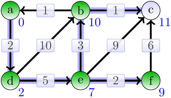
Suppose that the edges are relaxed in the following order: $ \Tuple{a, d} $, $ \Tuple{b, a} $, $ \Tuple{b, c} $, $ \Tuple{d, b} $, $ \Tuple{d, e} $, $ \Tuple{e, b} $, $ \Tuple{e, c} $, $ \Tuple{e, f} $, $ \Tuple{f, c} $. The graphs below show the estimates and the constructed shortest paths (the highlighted edges) after each loop iteration. After the first iteration, the estimates of many (but not all) vertices are accurate. For instance, as the edge $ \Tuple{a, d} $ was relaxed before $ \Tuple{d, e} $ and a shortest path from $ a $ to $ e $ is $ \Path{a,d,e} $, the estimate of $ e $ is already accurate.

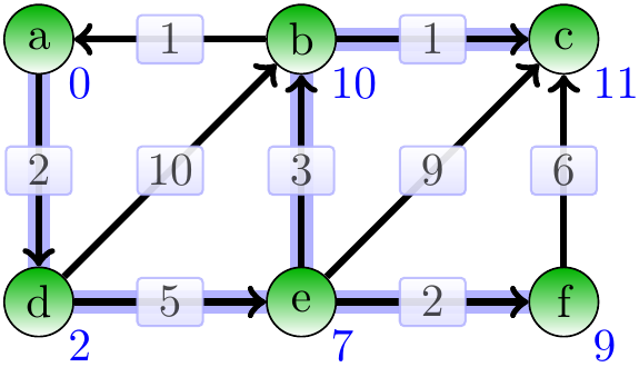
After the second iteration, all the estimates are accurate and nothing will change during the following iterations.

Observe that with an optimal edge relaxation order, only one iteration would have been enough. One such order is the following: $ \Tuple{a, d} $, $ \Tuple{d, e} $, $ \Tuple{e, f} $, $ \Tuple{e, b} $, $ \Tuple{b, c} $, $ \Tuple{b, a} $, $ \Tuple{d, b} $, $ \Tuple{e, c} $, $ \Tuple{f, c} $.

Example: Applying Bellman-Ford, negative-weight edges

Consider again the graph below having a negative-weight edge but no negative-weight cycles.

The graphs below show the estimates and the constructed shortest paths (the highlighted edges) after each loop iteration. After the first iteration:

After the second iteration:

After the third iteration:

The situation is stabilized already after the third iteration. Here the edges were relaxed in the following order: $ \Tuple{c, d} $, $ \Tuple{b, c} $, $ \Tuple{a, c} $, $ \Tuple{a, b} $, $ \Tuple{c, e} $.

Again, with an optimal edge relaxation order, only one iteration would have been enough. Such an ordering is: $ \Tuple{a,c} $, $ \Tuple{a,b} $, $ \Tuple{b,c} $, $ \Tuple{c,e} $, $ \Tuple{c,d} $.

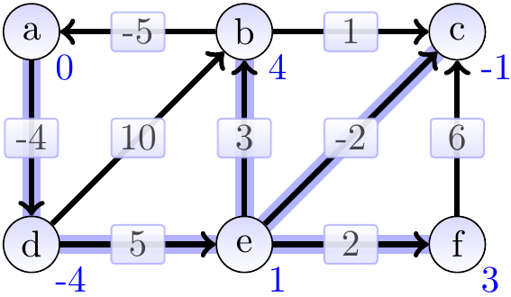
Example: Applying Bellman-Ford, negative-weight cycles

Consider the graph below, the vertex annotations showing the estimates in the beginning.

The graphs below show the estimates and the constructed shortest paths (the highlighted edges) after each loop iteration. After 1st iteration:

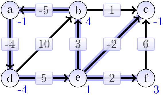
After 2nd iteration:

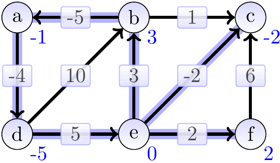
After 3rd iteration:

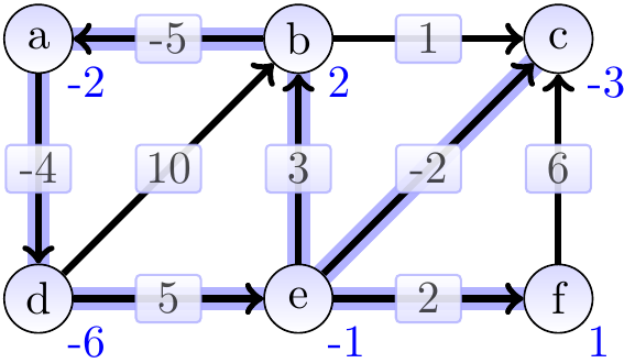
After 4th iteration:

After 5th iteration:

After 6th iteration:

At the end, $ \SPEst{a} + \Weight{a}{d} = -3 + -4 = -7 < \SPEst{d} = -6 $, indicating the existence of a negative-weight cycle.

Observe that we can find a negative cycle by finding a cycle (use Depth-first search) in the sub-graph consisting only of the predecessor edges (the highlighted edges in the figure).

What is the worst-case running time of the algorithm?

Initialization takes time $ \Oh{\NofV} $.
The first for-loop is iterated $ \NofV-1 $ times, each iteration taking time $ \Oh{\NofE} $.
The second for-loop is iterated at most $ \NofE $ times, each iteration taking a constant time.

The total running time is thus $ \Oh{\NofV \NofE} $.

Example: Finding currency trading arbitrage

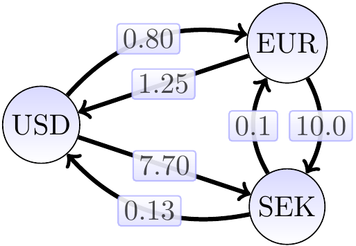
Suppose that we are given a set of exchange rates between some currencies. Is it possible to change money between the currencies so that we end up in having more in the original currency? That is, does the exchange rate graph have a cycle with the product of the edge weights more than 1? As an example, consider the exchange rate graph below.

The Bellman-Ford algorithm cannot be directly applied to finding such cycles because it considers the sums of edge weights, not products. However, we can use the following observation: a product $ x_1 x_2 \cdots x_n $ is greater than $ 1 $ when its logarithm is greater than $ 0 $. Now use

the equality $ \Lg(x_1 x_2 \cdots x_n) = \Lg(x_1) + \Lg(x_2) + … + \Lg(x_n) $, and
the fact that $ \Lg(x_1) + \Lg(x_2) + … + \Lg(x_n) > 0 $ when $ {-\Lg(x_1)} + {-\Lg(x_2)} + … + {-\Lg(x_n)} < 0 $.

Let’s thus replace each exchange rate $ \alpha $ with the value $ -\Lg{\alpha} $ rounded up a bit (in order to eliminate extremely small profits and rounding errors). The resulting graph has a negative-weight cycle iff the original graph has a possibility for arbitrage. Applying this to the exchange rate graph above, we get the graph below.

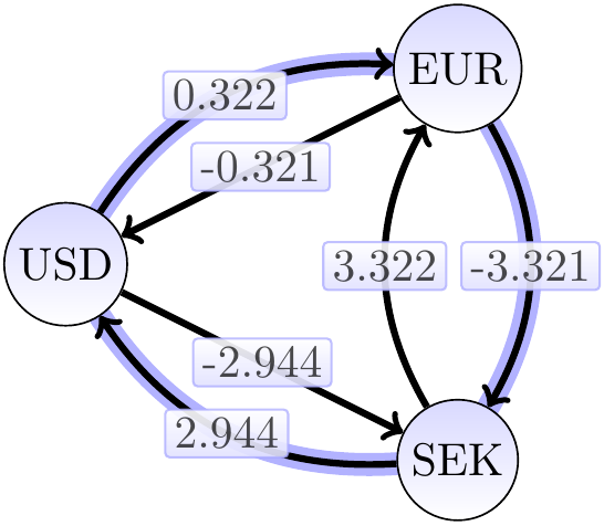
The negative cycle in the graph above (the highlighted edges) corresponds to an exchange sequence offering 4 percent profit as $ 0.8 \times 10.0 \times 0.13 = 1.04 $.

Single-source shortest paths on DAGs¶

For directed, acyclic edge-weighted graphs it is possible to obtain an ordering for the vertices so that relaxations can be done in an optimal order. The algorithm:

Disregarding the edge-weights, obtain a topological ordering for the graph (recall Section Topological sort).
Initialize the shortest-path weight estimates and predecessor attributes as usual.
Starting from the source vertex $ s $, perform relaxation in the topological order.

Since all the vertices on any path from the source to the current vertex have been considered when starting to relaxing the edges from the current vertex $ u $, $ \SPEst{u} = \SPDist{s}{u} $. A topological ordering can be computed in time $ \Oh{\NofV+\NofE} $. Thus the running time of the whole algorithm is thus $ \Oh{\NofV+\NofE} $.

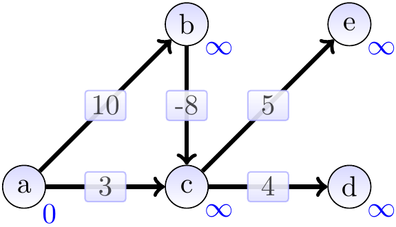
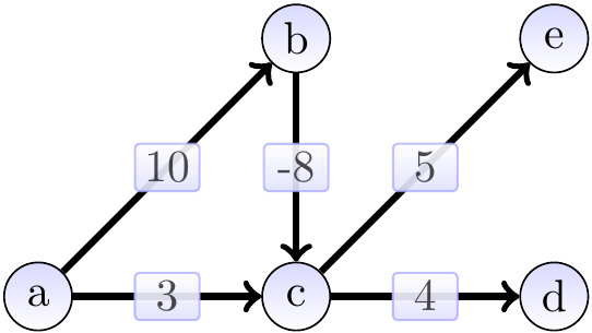
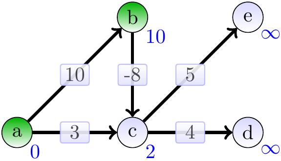
Example

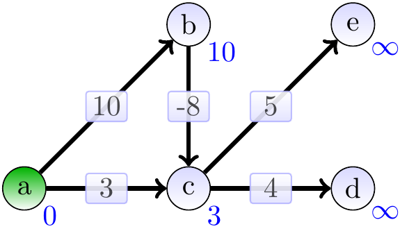
Consider the directed acyclic graph on the right. Note that it has negative-weight edges. A topological ordering for it is: $ a $, $ b $, $ c $, $ e $, $ d $.

Starting from the source vertex $ a $ and performing the relaxations in the topological order, we get the following steps. The start situation after initialization:

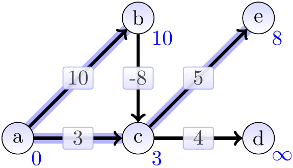
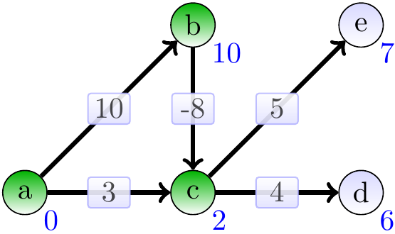
Include $ a $ and relax its neighbours:

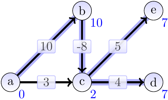
Include $ b $ and relax its neighbours:

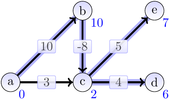
Include $ c $ and relax its neighbours:

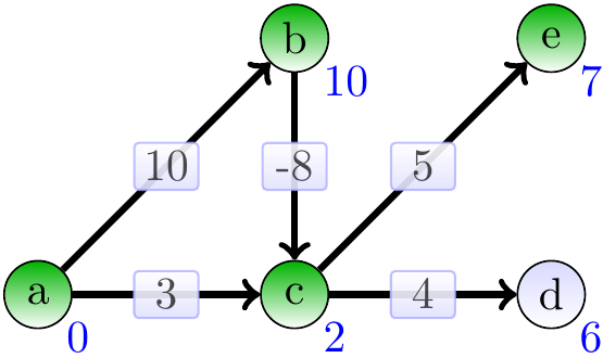
Include $ e $ and relax its neighbours:

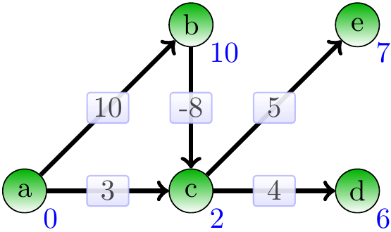
Include $ d $ and relax its neighbours:

Single-source shortest paths¶

Shortest-path weight estimates and relaxation¶

Dijkstra’s algorithm¶

The Bellman-Ford algorithm¶

Single-source shortest paths on DAGs¶

Further reading¶