Binary search trees
In this round, we implement ordered sets and maps with Binary trees having some special properties. We associate the keys to nodes and the key of a node \( \TNode \) is denoted by \( \TKeyOf{\TNode} \).
Definition: Binary search tree
A binary tree is a binary search tree (BST) if the following binary search tree property holds: For every node \( \TNode \) in the tree it holds that
if \( \TNodeI \) is a node in the sub-tree rooted at the left child of \( \TNode \), then \( \TKeyOf{\TNodeI} \le \TKeyOf{\TNode} \)
if \( \TNodeI \) is a node in the sub-tree rooted at the right child of \( \TNode \), then \( \TKeyOf{\TNodeI} \ge \TKeyOf{\TNode} \)
We assume that the keys are distinct; for equal keys discussion, see Problem 12.1 in Introduction to Algorithms, 3rd ed. (online via Aalto lib). For simplicity, we mainly focus on ordered sets in these notes, ordered maps are a relatively straightforward extension (each node also contains the value to which the key is mapped).
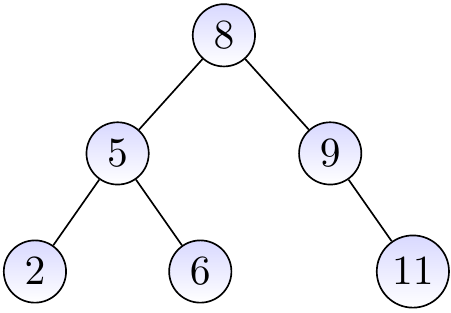
Example
The three binary trees below are BSTs.
The binary tree below is not a BST as the node with the key \( 4 \) is in the right sub-tree of the root node having the key \( 8 \).
Searching keys
Searching a key \( k \) in a BST is easy due to to the binary search tree property. We traverse the nodes recursively, starting from the root, and proceed as follows:
If the current node \( x \) has the key \( k \), we are done.
If the key in the node \( x \) is greater than \( k \),
traverse the left child of the node if it has one, or
report that the key is not in the BST if the node has no left child.
If the key in the node \( x \) is less than \( k \),
traverse the right child of the node if it has one, or
report that the key is not in the BST if the node has no right child.
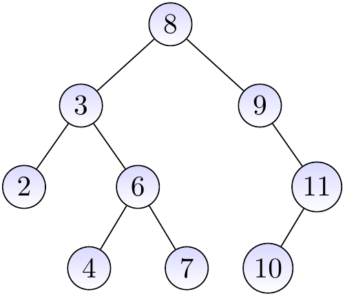
Example
Consider again the BST below.
If we search for the key \( 4 \),
we start from the root and note that \( 8 > 4 \),
go to the left child and note that \( 3 < 4 \),
go to the right child and note that \( 6 > 4 \),
go to the left child and note that \( 4 = 4 \), and
report that \( 4 \) is in the tree.
Example
Consider again the BST below:
If we search for the key \( 5 \),
we start from the root and note that \( 8 > 5 \),
go to the left child and note that \( 3 < 5 \),
go to the right child and note that \( 6 > 5 \),
go to the left child and note that \( 4 < 5 \), and
note that the node does not have a right child and thus report that \( 5 \) is not in the tree.
Inserting keys
To insert a new key in a BST, first proceed like when searching for the key. If the key is already in the BST, stop. Otherwise, the last step in search procedure wanted to traverse the non-existing left (or right, respectively) child of a node \( n \). In this case,
insert a new node \( n’ \) with the key \( k \) in the tree, and
make it to be the left (right, respectively) child of \( n \).
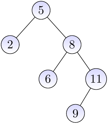
Example
Consider again the BST below.
If we insert the key \( 10 \) in the tree, we
start from the root and note that \( 8 < 10 \),
go to the right child and note that \( 9 < 10 \),
go to the right child and note that \( 11 > 10 \),
note that the node does not have a left child, and
add \( 10 \) as the left child of \( 11 \).
The resulting BST is shown below.
Removing keys
Removing keys is a bit more complicated. First, find the node \( z \) having the key. Then:
If the node \( z \) is a leaf, we just remove it.
If the node \( z \) has only one child \( x \), remove the node \( z \) and substitute the only child \( x \) to be in its place.
Otherwise, the node \( z \) has two chilren. In this case, we
find the node \( y \) with the largest key in the left subtree of \( z \),
make \( z \) have the key of \( y \),
remove the node \( y \) and substitute the left child \( x \) of \( y \) (if it has one) to be in its place. Note that \( y \) does not have a right child; why?.
A task: study the following examples and argument to yourself why the BST property is preserved when we remove keys with the above method. That is: if the tree is a BST in the beginning, then the tree resulting after the key removal is also a BST.
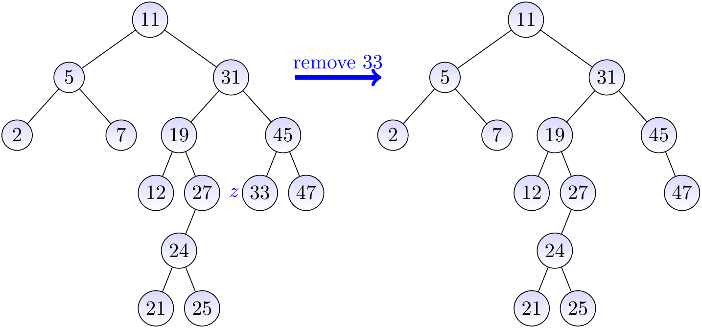
Example
Let us remove the key 33 from the BST on the left-hand side below. In this case, we simply remove the node \( z \) having the key 33. The result is shown on the right hand side.
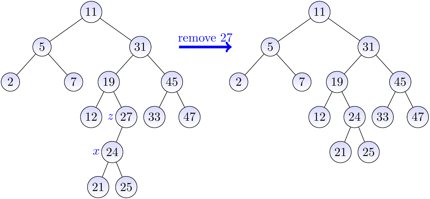
Example
Let us remove the key 27 from the BST on the left-hand side below. In this case, we remove the node \( z \) having the key 27 and move its only child \( x \) to be in its place.
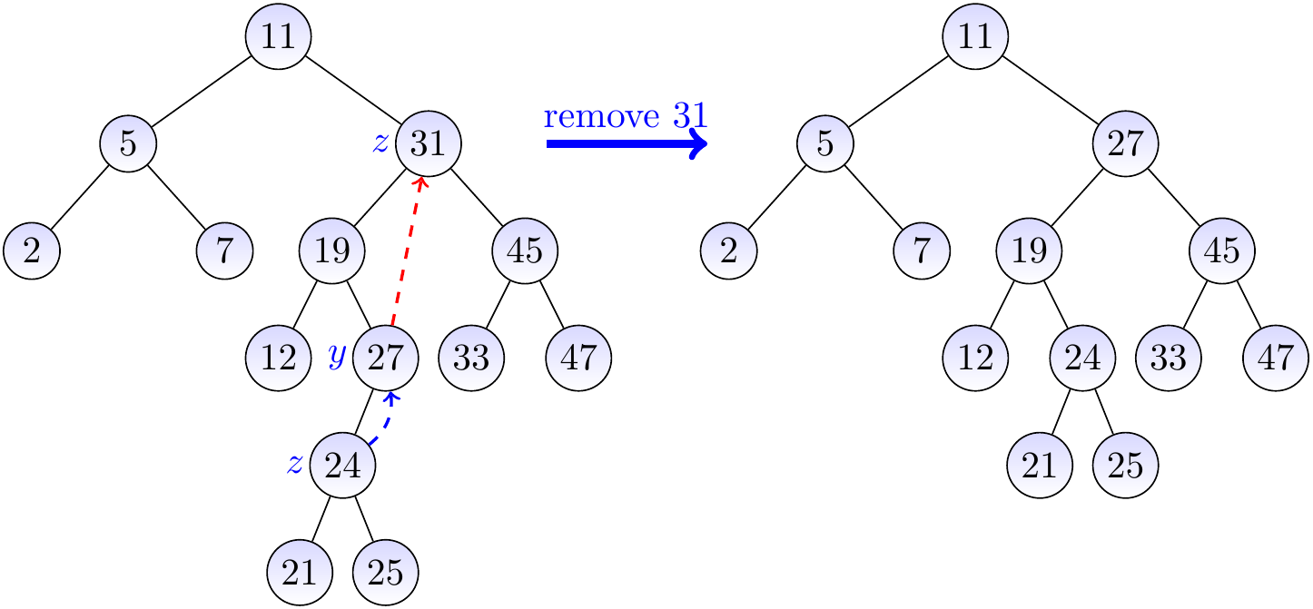
Example
Let us remove the key 31 from the BST on the left-hand side below.
As the node \( z \) with the key 31 has two children, we find the node \( y \) with the largest key in the left sub-tree of \( z \).
We then move the key 27 of \( y \) to be the key of \( z \), shown with the red arrow in the figure.
After this, we remove the node \( y \) and move its only child \( x \) to be in its place (shown with the blue dashed arrow).
Listing the keys in ascending order
Due to the BST property, listing the elements/keys in ascending order is easy: just traverse the tree in inorder (recall the Section Traversing trees) and output the key of the node when it is visited. Thus \( n \) elements could be sorted by (i) inserting them one-by-one in a BST, and (ii) then listing the elements at the end. However, this would not be the most efficient sorting algorithm available.
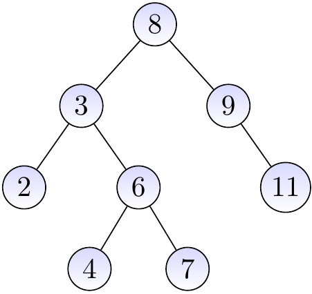
Example
Consider the BST below. Traversing the nodes in inorder and printing the keys gives the sequence 2,3,4,6,7,8,9,10,11 as expected.
Finding the smallest and largest keys
The smallest key can be found by simply iteratively traversing, starting from the root, to the left child as long as possible. Similarly, the largest key can be found from the “rightmost” node.
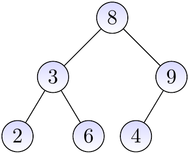
Example
Consider the BST shown below. The smallest key in it is 2 and the largest one is 11.
Finding the predecessor and successor keys
Given a key \( k \), the predecessor key in a BST is the largest key
that is smaller than \( k \) or
“None” if all the keys in the BST are at least as large as \( k \).
It can be found by initializing a variable best to “None” and
traversing the tree from the root node as far as possible:
If the key \( k’ \) in the current node is \( k \) or larger, go to the left child.
Otherwise, set
bestto \( k’ \) and go to the right child.
At the end, report best.
Finding the successor key of \( k \) (the smallest key that is larger than \( k \))
can be done in a similar way.
Example
Consider the BST shown below.
The predecessor key of \( 5 \) is \( 4 \).
The predecessor key of \( 20 \) is \( 11 \).
The predecessor key of \( 2 \) is “None”.
The successor key of \( 4 \) is \( 6 \).
Time-complexity analysis
The algorithms for searching and inserting keys, as well as finding predecessor and successor keys,
only traverse one path in the tree and
perform constant-time operations in each traversed node (assuming that key comparison can be done in constant time).
Thus their time-complexity is \( \Oh{h} \), where \( h \) is the height of the tree.
The algorithm for removing keys also traverses one path to find the removed key and then continues one path downwards to find the key that is substituted in its place. Thus its time-complexity is also \( \Oh{h} \).
Expected and worst-case behaviour
It can be shown that if one builds a BST from \( n \) random distinct keys, then the expected height of the BST is \( \Oh{\Lg n} \), see Section 12.4 in the Introduction to Algorithms, 3rd ed. (online via Aalto lib) book. However, it is also easy to insert keys in a way that makes the tree very inbalanced and look like a linked list.
Example
Inserting the keys 1, 2, 3, 4, and 5 in this order gives the BST shown below. This is essentially a linked list (the right child link corresponds to the next element link in linked lists).
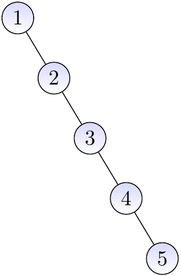
Thus the worst-case time complexity of the operations given earlier is \( \Theta(n) \) when the tree has \( n \) keys.
In the following sections, we show how to fix this worst-case situation by balancing BSTs so that searching, inserting, and deleting keys can be done in time \( \Oh{\Lg n} \) in the case the tree has \( n \) keys in it.