Red-Black Trees¶

Red-black trees are another form of balanced binary search trees. In them, only one “color” bit of additional memory is required for each node. They are used in many libraries to implement ordered sets and maps. For instance:

In Scala, both the mutable TreeMap as well as the immutable TreeMap classes provide ordered maps implemented with red-black trees.
In Java, java.util.TreeMap implements mutable ordered maps with red-black trees. Similarly, java.util.TreeSet uses TreeMap to implement ordered sets.
In the C++ standard library implementations, map and set classes are usually implemented with red-black trees.

See, for instance, this external visualization tool for red-black trees to see how red-black trees work.

Definition: Red-black trees

A binary search tree is a red-black tree if

each node in it is colored either red or black,
the root node is black,
if a node is red, the both its children are black, and
for each node, all simple paths from the node to the descendant leaves contain the same number of black nodes.

Example

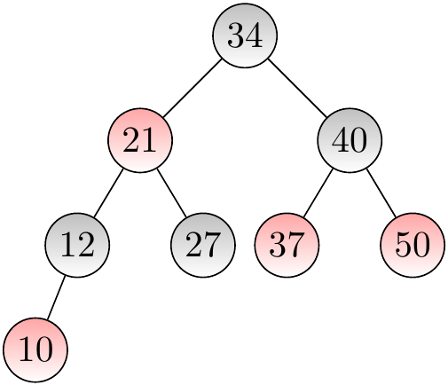
The tree below is a red-black tree.
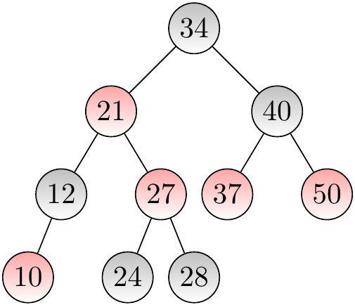
The BST below is not a red-black tree as it violates the requirement 3.
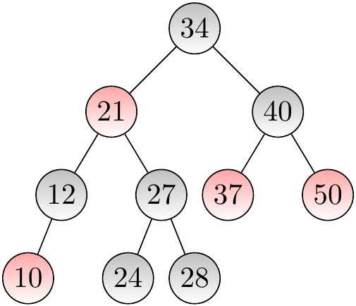
The BST below is not a red-black tree as it violates the requirement 4.

The red nodes allow a certain degree of inbalance but not too much as a path cannot have two successive red nodes.

Lemma: 13.1 in Cormen et al

A red-black tree with \( n \) nodes has height at most \( 2 \Lg(n+1) \).

As red-black trees are BSTs, searching and listing the keys in a tree is done as with non-balanced basic BSTs. Thus searching for keys and finding predecessor and successor keys in a red-black tree are logarithmic time operations.

As with AVL Trees, we only have to show how we can insert and remove keys in red-black trees. Again, the basic insertion and removal is as with basic BSTs but we then have to “rebalance” the tree to make it red-black again.

Inserting keys¶

The first phase in inserting a key in a red-black tree works as in basic BSTs. The new leaf node is initially colored red, and then:

If its parent is black, the new tree is still a red-black tree and we are done.
If the parent is red, the third condition of red-black trees is violated and we have to “rebalance”.

To consider the latter case above, we now

assume that a node \( z \) has just been made red and its parent \( p \) is also red, and
then show how to rebalance the tree upwards until it is a valid red-black tree.

For simplicity, we only present rebalancing for the case when \( z \) is in the left sub-tree of its grandparent; the right sub-tree case is symmetric.

Rebalancing, case I¶

In this case also the sibling \( u \) of \( p \) (the “uncle” of \( z \)) is red. The sub-trees rooted at the nodes \( c_1 \), \( c_2 \), \( b \), \( u_1 \) and \( u_2 \) are valid red-black trees in which all the paths from the sub-tree roots to leaves contain \( k \) black nodes.

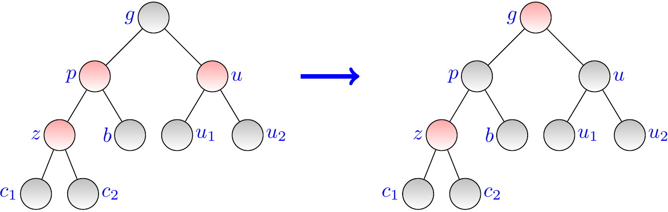
To rebalance in this case, color \( g \) red and \( p,u \) black. The sub-tree rooted at \( g \)

is now an otherwise valid red-black tree except that its root is red, and
all the paths from \( g \) to leaves contain \( k+1 \) black nodes as was the case before the recoloring.

Now, if \( g \) is the root of the whole tree, color it black and stop. Otherwise, continue rebalancing upwards if the parent of \( g \) is red.

Rebalancing, case II¶

In this case, the sibling \( u \) of \( p \) (the “uncle” of \( z \)) is black, and \( z \) is the left child of \( p \). The subtrees rooted at the nodes \( c_1 \), \( c_2 \), \( b \), and \( u \) are valid red-black trees in which all paths from the sub-tree root to leaves contain the same number of black nodes.

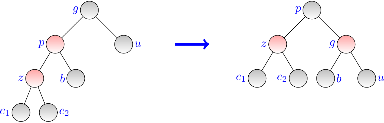
To rebalance, rotate the grandparent \( g \) right and color \( p \) black and \( g \) red. The new sub-tree rooted at \( p \)

is now a valid red-black tree, and
all the paths from \( p \) to leaves contain the same equal number of black nodes as from \( g \) before the rotation and recoloring.

We are now done with rebalancing.

Rebalancing, case III¶

In this case, te sibling \( u \) of \( p \) (the “uncle” of \( z \)) is black, and \( z \) is the right child of \( p \). The subtrees rooted at the nodes \( c_1 \), \( c_2 \), \( b \), and \( u \) are valid red-black trees in which all paths from the sub-tree root to leaves contain the same number \( k \) of black nodes.

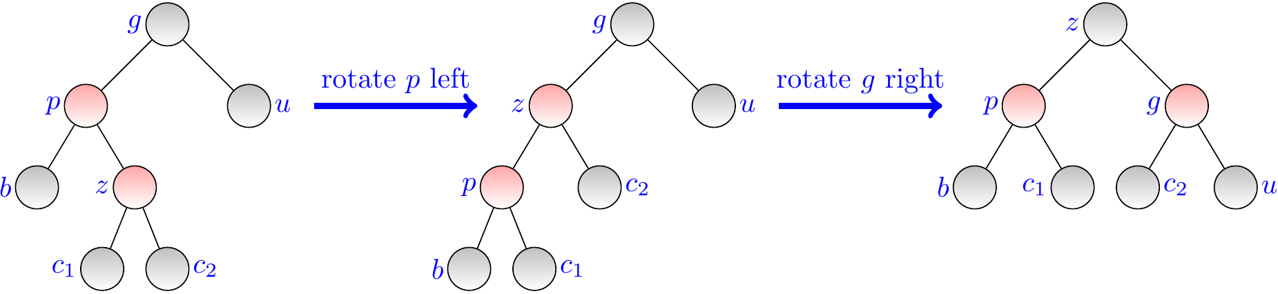
To rebalance,

first rotate the parent \( p \) left, and
then rotate the grandparent \( g \) right and color \( z \) black and \( g \) red.

The new sub-tree rooted at \( z \)

is now a valid red-black tree, and
all the paths from \( z \) to leaves contain \( k+1 \) black nodes, as was the case from \( g \) before the rotations and recoloring.

We are done with rebalancing.

Removing Keys from Red-Black Trees¶

Again, as with basic BSTs and AVL trees, removing keys is a bit more complicated. The basic process is as with basic BSTs. If the removed node was red, there is no need for rebalancing. But when we remove a black node, the “black height” of a sub-tree rooted in the substituting node of the tree is decreased by one and we must rebalance. The details on how to do this can be found in Section 13.4 of Introduction to Algorithms, 3rd ed. (online via Aalto lib), they are not included in the course.