AVL Trees¶

AVL trees are one form of height-balanced BSTs. The name “AVL” comes from the names Georgy Adelson-Velsky and Evgenii Landis, who presented the data structure in

G. M. Adel’son-Vel’skii and E. M. Landis, An algorithm for organization of information, Dokl. Akad. Nauk SSSR 146(2):263–266, 1962.

The definition is as follows:

Definition

A binary search tree is an AVL tree if, for each node \( x \) in it, it holds that the heights of the left and right sub-tree of \( x \) differ by at most one.

Example

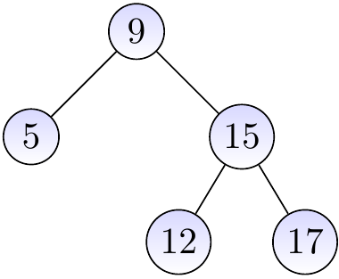
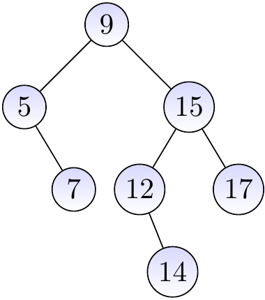
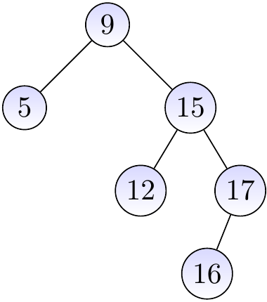
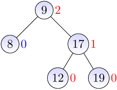
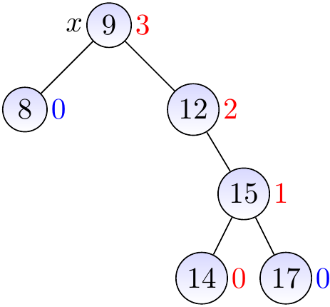
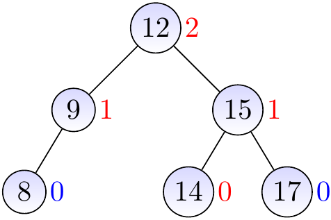
The two BSTs below are AVL trees.
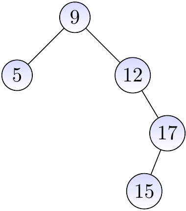
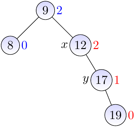
The BST below is not an AVL tree as the AVL property is not holding in the node with the key 12: its left sub-tree is empty and has height -1 while the right sub-tree has height 1.
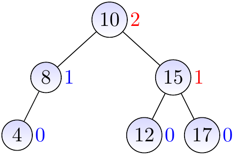
The BST below is not an AVL tree as the left child of the root has height 0 and the right one has height 2

If we have an AVL tree of height \( h \), how many nodes does it at least contain? This lower bound can be expressed as recurrence \( T(h) \) with

\( T(-1) = 0 \) and \( T(0) = 1 \)
\( T(h) = 1 + T(h-1) + T(h-2) \) for \( h \ge 2 \).

Recall that the Fibonacci numbers \( F_n \) are defined by \( F_0 = 0 \), \( F_1 = 1 \) and \( F_n = F_{n-1}+F_{n-2} \) for \( n \ge 2 \). Therefore, \( T(h) > F_{h+1} \). As \( F_n \) is the closest integer to \( \frac{\varphi ^{n}}{\sqrt {5}} \) with \( \varphi = 1.618… \), an AVL tree of height \( h \) contains an exponential amount of nodes with respect to the height \( h \) of the tree. Thus the height of an AVL tree with \( n \) nodes is logarithmic to \( n \). Because of this fact,

searching keys and
finding the smallest and largest keys

can be done in logarithmic time in AVL trees. We now only have to show how inserting and removing keys can be done in logarithmic time as well. In both cases, the idea is to rebalance the tree after a local modification (insert or removal) so that the AVL property holds again. The rebalancing proceeds only upwards in the tree and thus works in logarithmic time as well when the tree had the AVL property before the modification.

Inserting Keys¶

The first phase in inserting keys to an AVL tree works as with BSTs (recall the Section Inserting keys): we search the correct insertion place and insert a new leaf node \( z \) with the new key. But the height of the parent node \( p \) of \( z \), as well as its ancestors, may now have been increased by one and the AVL tree property does not necessarily hold anymore as there may be nodes whose other child has height two more than the other. Thus we have to rebalance the tree so that the AVL tree property holds again. We do this bottom-up, starting from the parent \( g \) of \( p \). (The AVL property already holds for the node \( p \), why?)

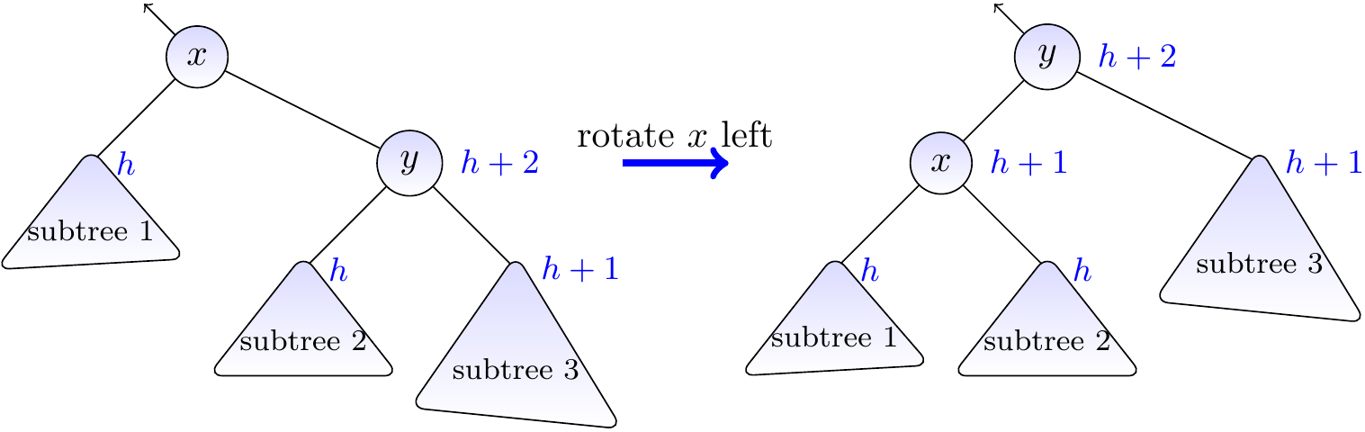
In general, we show how to rebalance the sub-tree rooted at a node \( x \) whose child \( y \) has height \( h+2 \) while the other child has height \( h \). It is assumed that the AVL property already holds for the sub-trees rooted at the children of \( x \). After rebalancing, the AVL property holds for the sub-tree. As the height of the sub-tree may have increased by one in the insertion, we then recursively check whether the parent of the sub-tree has to be rebalanced as well. For simplicity, we only present here the case when \( y \) is the right child of \( x \). The case of the left child is symmetric.

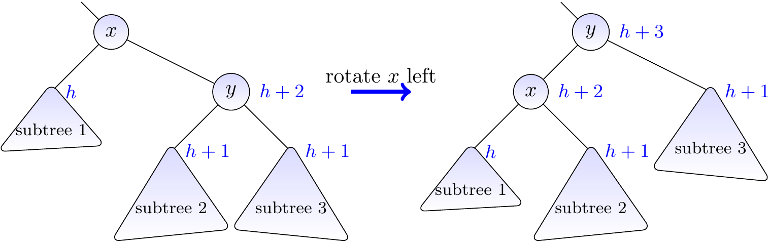
Case I: \( y \) is right-heavy¶

Recall that we assume that the sub-tree rooted at the right child \( y \) of \( x \) has height \( h+2 \) but that at the left child of \( x \) has height \( h \). In this first case, the height of the right sub-tree of \( y \) is \( h+1 \) and that of the left is \( h \). If we rotate \( x \) left, the sub-tree will be rooted now at \( y \) and the AVL property holds for it. This is illustrated in the figure below.

Example

Consider the AVL tree shown below.
Insert a new node with the key \( 19 \) and height 0.
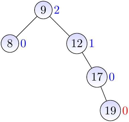
The parent is balanced, update its height to 1.
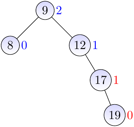
Observe that the next parent \( x \) is not balanced: its left sub-tree is empty and thus has height -1, while the right one has height 1. The right sub-tree of \( x \) at \( y \) is right-heavy.
Thus we rotate \( x \) left to make the sub-tree balanced.
We observe that the next parent (the root) is balanced.

Case II: \( y \) is neither left- or right-heavy¶

Again, the right sub-tree of \( x \) rooted at \( y \) has height \( h+2 \) but that at the left child of \( x \) has height \( h \). But in this case, the heights of the left and right sub-trees of \( y \) are both \( h+1 \). If we rotate \( x \) left, the sub-tree will be rooted now at \( y \) and the AVL property holds for it.

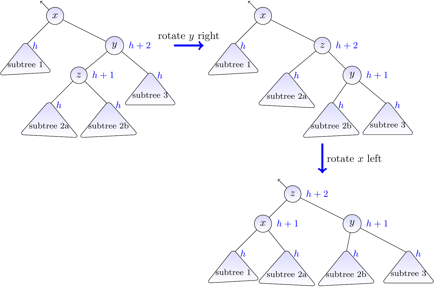
Case III: \( y \) is left-heavy¶

Again, the sub-tree of \( x \) rooted at \( y \) has height \( h+2 \) but that at the left child of \( x \) has height \( h \). In this case, the height of the left sub-tree of \( y \) is \( h+1 \) and that of the right is \( h \). To balance the sub-tree at \( x \),

we first rotate \( y \) right so that the right sub-tree of \( x \) becomes right-heavy, and
then proceed as above by rotating \( x \) left.

Example

Consider the AVL tree below.
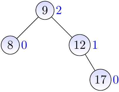
Insert a new node with the key \( 15 \) and height 0.
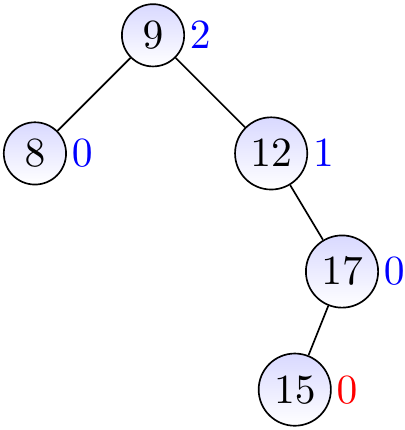
The parent is balanced, update its height to 1.
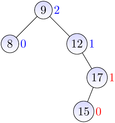
Observe that the next parent \( x \) is not balanced: its left sub-tree is empty and thus has height -1, while the right one has height 1. The right sub-tree at \( y \) is left-heavy.
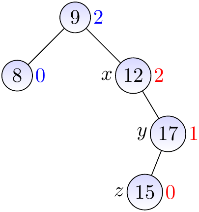
We thus first rotate \( y \) right to make the right sub-tree of \( x \) right-heavy…
and then the rotate \( x \) left to make the sub-tree balanced. Finally, we observe that the next parent (the root) is balanced.

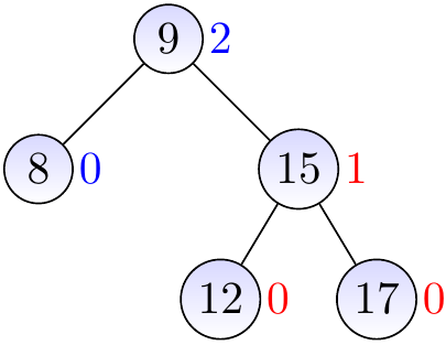
Example

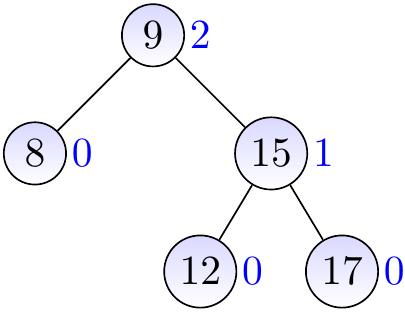
Consider the AVL tree drawn below.
We insert a node with the key \( 14 \) and height 0.
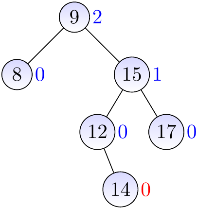
We observe that the parent and the grandparent are balanced and update their heights. We next observe that the next parent \( x \) is not balanced: its left sub-tree has height 0 while the right one has height 2. Furthermore, the right sub-tree at \( y \) is left-heavy.
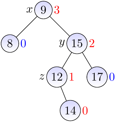
We rotate \( y \) right to make the right sub-tree of \( x \) right-heavy, and …
then the rotate \( x \) left to make the sub-tree (and the whole tree) balanced.

Removing keys¶

The basic removal process is as with unbalanced BSTs (recall Section Removing keys). But when we remove a node, the height of its parent node and all its ancestors can decrease by one. Again, this creates an inbalance of at most two in the heights of sub-trees and we can use the above rebalancing techniques to restore the AVL property.

Example

Consider the AVL tree shown below.
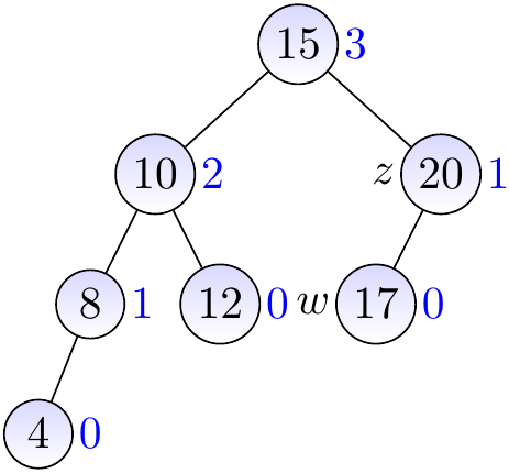
When we remove the key \( 20 \), we remove the node \( z \) and substitute \( w \) in its place. We now observe that the parent \( x \) is unbalanced and its left child \( y \) is left-heavy.
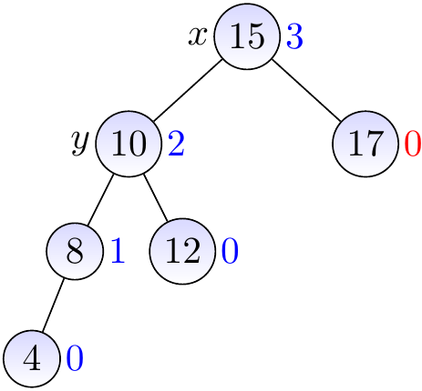
We thus rotate \( x \) right to regain the balance.