Balancing Binary Search Trees¶

We can make the search, insert, and remove operations to work in time \( \Oh{\Lg n} \), where \( n \) is the number of the keys in the tree, by balancing the trees. Balancing ensures that the height of the BST is \( \Oh{\Lg n} \). Many variants of balanced BSTs have been proposed, see, for instance, this wikipedia link. In the following sections, we’ll see

AVL trees, which were the first balanced BSTs, and
red-black trees, which are commonly used in many standard libraries.

However, we first show the key technique used in balancing both of these BST classes: rotations.

Rotations¶

A common operation used when balancing BSTs is rotation.

In left rotation of a node \( x \) with a right child \( y \), we transform the sub-tree rooted at \( x \) so that
- \( y \) becomes the root of the sub-tree,
- \( x \) becomes the left child of \( y \), and
- the left child of \( y \) becomes the right child of \( x \).
The right rotation is the dual operation for a node with a left child.

The figure below shows the rotattions graphically. The shaded triangles denote sub-trees and can be empty.

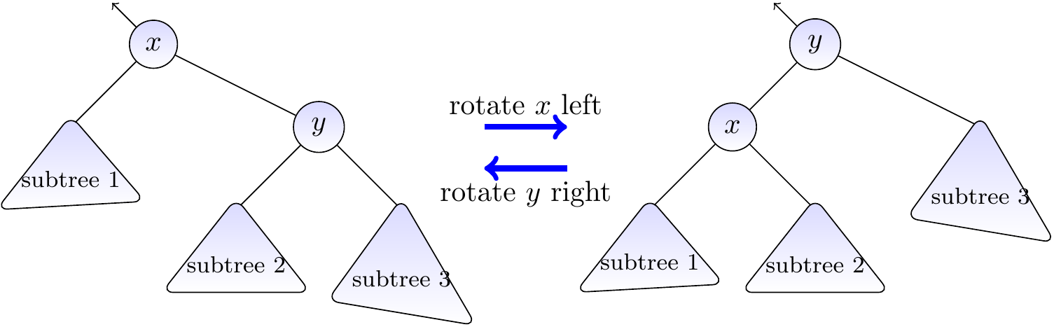
A key fact is that the left and right rotations preserve the BST property: If the BST property holds before a rotation, then it holds after the rotation. We can see this from the figure above for left rotation as follows:

Traversing the nodes in the subtree in inorder before the left rotation gives the keys in subtree 1, that of \( x \), those in subtree 2, that of \( y \) and those in subtree 3.
Traversing the nodes in the subtree in inorder after the left rotation gives the keys in subtree 1, that of \( x \), those in subtree 2, that of \( y \) and those in subtree 3.

A similar analysis can be performed for the right rotation.