Strongly Connected Components¶

Finding the strongly connected components of a directed graph is another algorithm based on Depth-first search. For a directed graph \( \Graph = \Tuple{\Verts,\Edges} \), a strongly connected component, or simply an SCC, is a maximal subset \( \SCC \subseteq \Verts \) such that for all the vertices \( u,v \in \SCC \), it holds that \( v \) is reachable from \( u \) and \( u \) is reachable from \( v \). Thus each cycle in a directed graph is inside an SCC. Vertices that are not in any cycle form their own unit components.

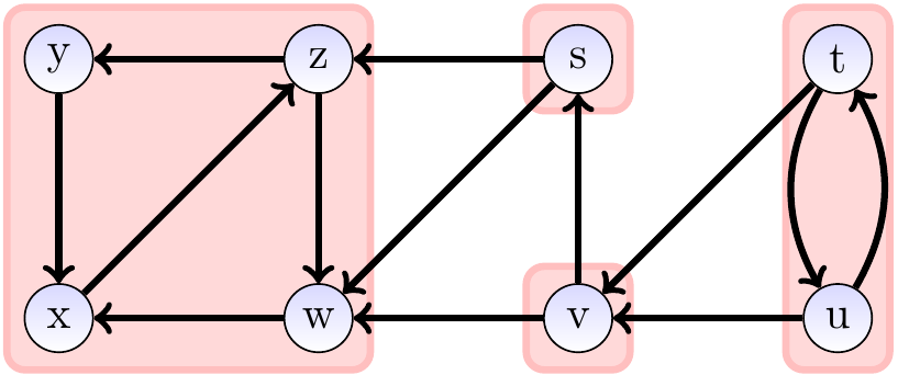
Example

Consider the graph shown below. Its strongly connected components, shown with the red areas, are \( \Set{s} \), \( \Set{t,u} \), \( \Set{v} \), and \( \Set{w,x,y,z} \).

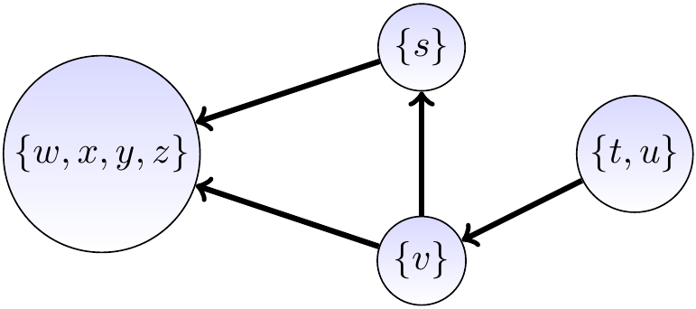
The component graph \( \GraphSCC = \Tuple{\VertsSCC,\EdgesSCC} \) of a directed graph \( \Graph \) is the directed graph where

the vertices \( \VertsSCC \) are the connected components of \( \Graph \), and
there is an edge \( \Tuple{\SCC,\SCC’} \in \VertsSCC \) from a component vertex \( \SCC \) to a different component vertex \( \SCC’ \) if \( \Tuple{u,v} \) is an edge in \( \Graph \) for some \( u \in \SCC \) and \( v \in \SCC’ \).

The component graph is acyclic. Why?

Example

Consider again the graph shown in the previous example. Its component graph is shown below.

There are several linear time, meaning \( \Oh{\Card{V}+\Card{E}} \) in this context, algorithms for computing the SCCs of a directed graph \( \Graph = \Tuple{\Verts,\Edges} \), see e.g. this Wikipedia article. The following presents a variant of Kosaraju’s algorithm. It uses depth-first search twice:

Perform depth-first search on the original graph to obtain the visit time-stamps.
Make the transpose \( \GraphT \) of the graph \( \Graph = \Tuple{\Verts,\Edges} \) by reversing the directions of the edges: \( \GraphT = \Tuple{\Verts, \EdgesT} \), where \( \EdgesT = \Setdef{\Tuple{u,v}}{\Tuple{v,u} \in \Edges} \).
Perform depth-first search on the transpose graph \( \GraphT \) but start the sub-searches from the vertices in the reverse order of the finish time-stamps produced by the first depth-first search.

The SCCs are the nodes in the depth-first search forests produced by the second depth-first search.

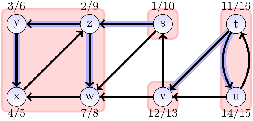
Example

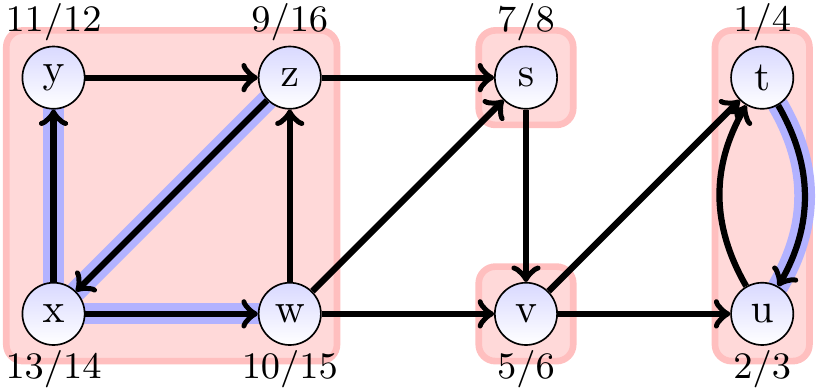
Consider the graph drawn below. Its strongly connected components are \( \Set{s} \), \( \Set{t,u} \), \( \Set{v} \), and \( \Set{w,x,y,z} \). Also shown in the graph are the time-stamps and the tree edges obtained by performing a depth-first search on the graph.

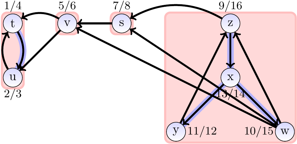
The transpose of the graph above is shown below. Observe that the SCCs of the transpose are the same as those of the original graph. Similarly, the component graph is again a DAG but transposed.

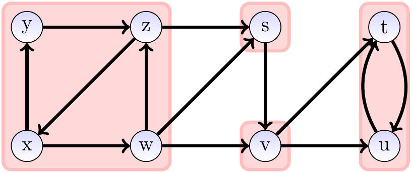
The graph below shows the result of applying depth-first search on the transpose graph in the reverse order of the finish time-stamps of the first depth-first search.

The sub-search starting from \( t \) finds the “leaf component” \( \Set{t,u} \)
The sub-search from \( v \) discovers the unit component \( \Set{v} \)
The sub-search from \( s \) discovers the unit component \( \Set{s} \)
The sub-search from \( z \) discovers the “root component” \( \Set{w,x,y,z} \)

The same graph but drawn in a different order in order to illustrate the order in which the components are found:

Why does this algorithm work? Below is a rough sketch, a more complete proof can be found in the book Introduction to Algorithms, 3rd ed. (online via Aalto lib).

The first depth-first search gives, in the finish time-stamps, a reverse topological sorting for the SCCs in the component graph.
The component graph of the transpose graph is the transpose of the component graph of the original graph.
Performing the second depth-first search on the transpose graph in the reverse topological order given by the first depth-first search
- first finds a component that does not have any successors in the transpose component graph,
- then finds a component that does not have any successors or whose successors have already been found in the transpose component graph,
- and so on.