Representations¶

In order to reason about graphs with algorithms, one has to represent graphs in the memory of a computer. First, observe that an undirected graph with $ n $ vertices can have at most $ \frac{n(n-1)}{2} $ edges, and a directed graph can have at most $ n^2 $ edges. We say that a graph is sparse if its number of edges is small compared to this maximum number of possible edges, otherwise it is dense. Sparsity is not an exactly defined concept as there is no exact definition for the phrase “small compared to” above.

In the following, we give the two common representations for graphs:

adjacency matrices, which are mainly used for dense graphs, and
adjacency lists, the most commonly used representation form.

In both of these representations, the $ n $ vertices in the graph are usually assumed to be the integers $ \Set{0,1,…,n-1} $ so that indexing is easy. If more complex vertex names such as strings are to be used, one can maintain a mapping from these to small integers so that the small integers can be used inside the graph algorithms. In the examples, we use symbolic names such as “$ a $” for better human readability.

Adjacency matrices¶

The adjacency matrix of a directed graph $ \Graph=\Tuple{\Set{0,1,…,n-1},\Edges} $ is a $ n \times n $ binary matrix $ A = (a_{u,v}) $ such that the entry $ a_{u,v} $ is $ 1 $ if $ \Tuple{u,v}\in\Edges $ and $ 0 $ otherwise. The matrix is easy to store in a row-by-row bit-vector of length $ n^2 $ (an array with $ \Ceil{\frac{n^2}{32}} $ 32-bit integers). In such bit-vector, the entry $ a_{u,v} $ can be found at the index $ un+v $.

Example: A directed graph and its adjacency matrix representation

Consider the directed graph shown below.

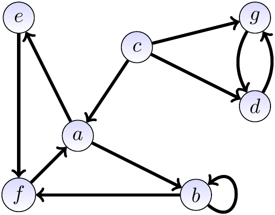
Its adjacency matrix representation is $$\begin{array}{c|ccccccc} & a & b & c & d & e & f & g\\ \hline a & 0 & 1 & 0 & 0 & 1 & 0 & 0\\ b & 0 & 1 & 0 & 0 & 0 & 1 & 0\\ c & 1 & 0 & 0 & 1 & 0 & 0 & 1\\ d & 0 & 0 & 0 & 0 & 0 & 0 & 1\\ e & 0 & 0 & 0 & 0 & 0 & 1 & 0\\ f & 1 & 0 & 0 & 0 & 0 & 0 & 0\\ g & 0 & 0 & 0 & 1 & 0 & 0 & 0 \end{array}$$ As a bit-vector, the matrix is $ 0100100 0100010 1001001 0000001 0000010 1000000 0001000 $.

The adjacency matrix of an undirected graph $ \Graph=\Tuple{\Set{0,1,…,n-1},\Edges} $ is simply the upper right half of the matrix: with $ 0 \le u < v < n $, the entry $ a_{u,v} $ is $ 1 $ if $ \Set{u,v}\in\Edges $ and $ 0 $ otherwise. If the matrix is presented as a row-by-row bit-vector, then the entry $ a_{u,v} $ can be found at the index $ un-\frac{u(u+1)}{2}+(v-u-1) $.

Example: An undirected graph and its adjacency matrix representation

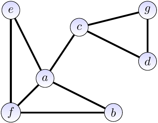
$$\begin{array}{c|ccccccc} & a & b & c & d & e & f & g\\ \hline a & & 1 & 1 & 0 & 1 & 1 & 0\\ b & & & 0 & 0 & 0 & 1 & 0\\ c & & & & 1 & 0 & 0 & 1\\ d & & & & & 0 & 0 & 1\\ e & & & & & & 1 & 0\\ f & & & & & & & 0\\ g & & & & & & & \\ \end{array}$$ As a bit vector, the matrix is $ 110110000101001001100 $ and the bit for the edge $ \Set{c,g} $ can be found at the index $ 2 \times 7 - \frac{2(2+1)}{2} + (6-2-1) = 14 - 3 + 3 = 14 $ under the mapping $ \left(\begin{smallmatrix}a&b&c&d&e&f&g\\0&1&2&3&4&5&6\end{smallmatrix}\right) $.

Some analysis:

Good for dense (and smallish) graphs.
Adding or removing an edge takes constant time.
Adding a new vertex is expensive as the whole matrix has to be expanded.
Graphs with many vertices take a lot of memory: the adjacency matrix for a directed graph with 1 million vertices would take over 100 gigabytes of memory.
Traversing the neighbors of a vertex is not very optimal if the degree of the vertex is low compared to the number $ n $ of all vertices as one has to go through all the $ n/8 $ bytes making the row.

Adjacency lists¶

In the adjacency list representation, each vertex is associated to a list of its neighbors. Naturally, a resizable array or a mutable set could be used instead of a list as well.

Example: A directed graph and its adjacency list representation

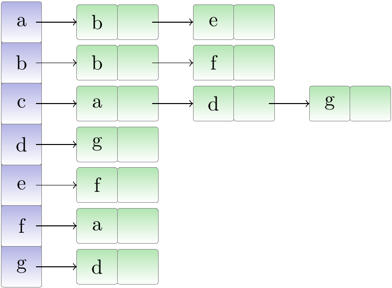
Consider the following directed graph.

An adjacency list representation for it is shown below.

Analysis:

Compact for sparse graphs: memory use is $ \Theta(\Card{\Verts}+\Card{\Edges}) $ instead of $ \Theta(\Card{\Verts}^2) $ use by the adjacency matrices.
Adding a new vertex is an amortized constant-time operation when dynamic arrays are used.
Adding and removing edges takes linear time in the degree of the vertex involved in the worst case.
Iterating over the neighbors of a vertex is easy.

The adjacency list representation is use more commonly than the adjacency matrix representation because in many applications the graphs tend to be both large and sparse.

Example: A directed graph and its adjacency list representation in a more compact form

It is also possible to represent the adjacency lists in an even more compact form by concatenating the neighbor lists into one array and indexing it with another array. As a concrete example, consider the directed graph

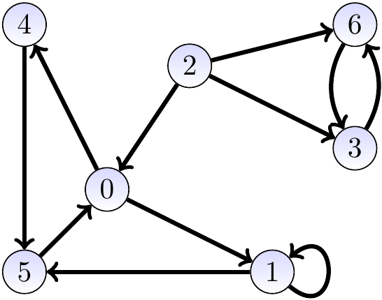
and the following representation

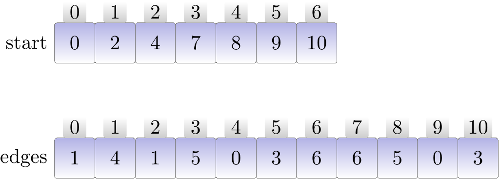
Now the vertices are $ \Set{0,1,…,6} $ and the neighbors of a vertex $ u $ can be found in the sub-array edges[start[$ u $]..start[$ u $+1]-1] or edges[start[$ u $]..edges.length-1] for the last vertex $ u=6 $.

In this representation method, the two arrays contain $ \Card{\Verts}+\Card{\Edges} $ integers in total. Of course, the drawback is that adding new vertices and edges is now more time consuming. Thus this representation should only be used when the graph is not modified often.

Representing vertex attributes¶

In many graph algorithms, we need to associate some data attributes to the vertices. There are multiple ways to achieve this but as/when the vertices are $ \Set{0,1,…,n-1} $, the easiest way is to have an array of $ n $ elements holding the attribute(s). From now on, we assume that accessing and setting a vertex attribute can be done in constant time.