Mathematical definitions
Graphs as mathematical structures are an important abstraction for reasoning about systems involving networks. Using a mathematical abstraction allows us to present algorithms in a context-independent way; for instance, a graph search algorithm can be applied to both social networks as well as to digital circuits.
Undirected Graphs
Mathematically, an undirected graph is a pair \( \Tuple{\Verts,\Edges} \), where
\( \Verts \) is a (usually finite) set of vertices, also called nodes, and
\( \Edges \) is a set of edges between the vertices. The elements in the set are pairs of the form \( \Set{u,v} \) such that \( u,v \in \Verts \) and \( u \neq v \). In this definition, edges between a vertex and itself, called self-loops, are thus forbidden.
The degree of a vertex is the number of edges incident to it; that is, the number of edges including the vertex.
Example
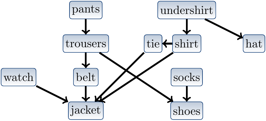
Consider the graph \( \Tuple{\Verts,\Edges} \) with
the vertices \( \Verts = \Set{a,b,c,d,e,f,g,h} \), and
the edges \( \Edges = \{\Set{a,b},\Set{a,c},\Set{a,e},\Set{a,f},\Set{b,f},\Set{e,f},\Set{c,d},\Set{c,g},\Set{d,g}\} \).
It is illustrated graphically below. The vertices drawn as circles and edges as lines between the vertices. The degree of the vertex \( a \) is 4.
A path of length \( k \) from a vertex \( v_0 \) to a vertex \( v_k \) is a sequence \( \Path{v_0,v_1,…,v_k} \) of \( k+1 \) vertices such that \( \Set{v_{i-1},v_i} \in \Edges \) for each \( i \in [1 .. k] \). A vertex \( v \) is reachable from a vertex \( u \) if there is a path from \( u \) to \( v \). Note that each vertex is reachable from itself as there is a path of length \( 0 \) from the vertex to itself. A path is simple if all the vertices in it are distinct. The graph is connected if every vertex in it is reachable from all the other vertices.
Example
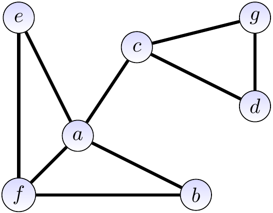
The graph below
has a non-simple path \( \Path{a,c,d,g,c,d} \) of length 5 from \( a \) to \( d \),
has a simple path \( \Path{a,c,d} \) of length 2 from \( a \) to \( d \), and
is connected but deleting the edge \( \Set{a,c} \) would make it disconnected.
A cycle is a path \( \Path{v_0,v_1,…,v_k} \) with \( k \ge 3 \) and \( v_0 = v_k \). A cycle \( \Path{v_0,v_1,…,v_k} \) is simple if \( v_1,v_2,…,v_k \) are all distinct. A graph is acyclic if it does not have any simple cycles.
Example
The graph below is not acyclic as it contains, among many others, a simple cycle \( \Path{a,e,f,a} \).
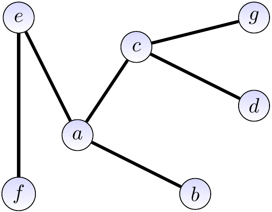
However, the graph below is acyclic.
Directed Graphs
Directed graphs are otherwise as undirected graphs except that the edges have a direction. Formally, a directed graph, or simply digraph, is a pair \( \Tuple{\Verts,\Edges} \), where
\( \Verts \) is a (usually finite) set of vertices, and
\( \Edges \subseteq \Verts \times \Verts \) is a set of edges between the vertices. A pair \( \Tuple{u,v} \in \Edges \) denotes an edge from the vertex \( u \) to the vertex \( v \).
Example
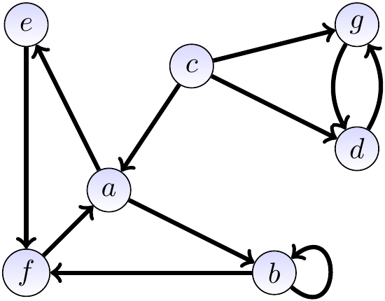
Consider the directed graph \( \Tuple{\Verts,\Edges} \) with
the vertices \( \Verts = \Set{a,b,c,d,e,f,g,h} \), and
the edges \( \Edges = \{\Tuple{a,b},\Tuple{a,e},\Tuple{b,b},\Tuple{b,f},\Tuple{c,a},\Tuple{c,d},\Tuple{c,g},\Tuple{d,g},\Tuple{e,f},\Tuple{a,f},\Tuple{g,d}\} \).
It is illustrated graphically below. Again, the vertices are drawn as circles. The edges are drawn as lines with direction arrow heads. Notice the loop from the vertex \( b \) to itself and the two edges between the vertices \( d \) and \( g \).
The out-degree of a vertex is the number of edges from it while the in-degree is the number of edges to it. A path of length \( k \) from a vertex \( u \) to the vertex \( u’ \) is a sequence \( \Path{v_0,v_1,…,v_k} \) of \( k+1 \) vertices such that \( v_0 = u \), \( v_k = u’ \) and \( \Tuple{v_{i-1},v_{i}} \in \Edges \) for all \( i \in [1 .. k] \). A path is simple if all vertices in it are distinct. A path \( \Path{v_0,v_1,…,v_k} \) is a cycle if \( k \ge 1 \) and \( v_0 = v_k \).
Example
In the directed graph shown below,
the in-degree of \( f \) is 2 and the out-degree is 1,
some simple paths are \( \Path{c} \), \( \Path{c,d,g} \), and \( \Path{a,b,f} \), while
the paths \( \Path{b,b} \), \( \Path{a,e,f,a} \), \( \Path{a,b,f,a} \), and \( \Path{d,g,d} \) are cycles.
Directed Acyclic Graphs (DAGs)
A directed acyclic graph, or simply a DAG, is a directed graph that does not contain any cycles. Such graphs arise in many applications, see, for instance, this Wikipedia page.
Example
DAGs arise naturally in many time- and order-related areas where something has to be done before something else can be done. In such a situation a cycle would mean that some things cannot be done at all. As a toy example, a dependency graph between clothes for dressing up is shown below (source: the Introduction to Algorithms, 3rd ed. (online via Aalto lib) book).