Basics of Analysis of Algorithms¶

We want our algorithms to be efficient, in a broad sense of using the given resources efficiently. Typical resources and properties of interest include

running time,
memory consumption,
parallelizability,
disk/network usage,
efficient use of cache (cache-oblivious algorithms),
and so on.

Naturally, we may have to make trade-offs. For instance, an algorithm that uses less memory may use more time than another algorithm.

In this course, we mainly focus on running time. We study the running time of a program/algorithm as a function $ f(n) $ in the size $ n $ of the input or some some other interesting parameter. Both $ n $ and $ f(n) $ are assumed to be non-negative. This allows us to find out how the performance of the algorithm scales when the parameter $ n $ grows. To this end, we perform two kinds of analysis:

Apriori analysis that studies the algorithm description and tries to find out how fast the running-time function $ f(n) $ grows when the parameter $ n $, such as the input size, grows. Is not interested in the exact values of $ f(n) $ but only the growth rate of $ f $. For instance, a linear-time algorithm is usually much better than a quadratic-time algorithm for the same computational task.
Experimental analysis, in which the exact running times of an implementation or many implementations are obtained, in a specific hardware and software setting, and then analyzed.

The Big O notation¶

As said above, in the apriori analysis are usually interested in the asymptotic growth rate of functions. Thus we use the Big O notation and its variants. It is a mathematical tool that abstracts away small values of $ n $ and constant factors. In the context of running time analysis of algorithms,

small values of $ n $ correspond to small inputs, and
constant factor variations in the running time are caused by the clock speed and architecture of the processor, memory latency and bandwidth, applied compiler optimizations etc.

Definition

For two functions, $ f $ and $ g $, we write $ f(n) = \Oh{g(n)} $ if there are constants $ c,n_0 > 0 $ such that $ f(n) \le cg(n) $ for all $ n \ge n_0 $.

If $ f(n) = \Oh{g(n)} $, then $ f(n) $ grows at most as fast as $ g(n) $ when we consider large enough values of $ n $. Note that the notation “$ = $” above is not the usual equality but is read as “is”. Thus $ f(n) = \Oh{g(n)} $ can be read “$ f(n) $ is big-O of $ g(n) $”. The notation $ f(n) \in \Oh{g(n)} $ would be mathematically more precise when $ \Oh{g(n)} $ is seen as a set of functions, see this wikipedia article. In addition to $ \BigOh $, one commonly also sees the following:

$ f(n) = \Omega(g(n)) $ if $ g(n) = \Oh{f(n)} $. When $ f(n) = \Omega(g(n)) $, we say that “$ f $ grows at least as fast as $ g $” or “$ f(n) $ is big-omega of $ g(n) $”.
$ f(n) = \Theta(g(n)) $ if $ f(n) = \Oh{g(n)} $ and $ g(n) = \Oh{f(n)} $. In such a case, we say that “$ f $ and $ g $ grow at the same rate” or “$ f(n) $ is big-theta of $ g(n) $”.

There are also “little-o” and “little omega”, although their use is not that common.

Definition

For two functions $ f $ and $ g $, we write $ f(n) = o(g(n)) $ if for every constant $ c > 0 $ there is a constant $ n_0 > 0 $ such that $ f(n) < cg(n) $ for all $ n \ge n_0 $.

If $ f(n) = o(g(n)) $, “$ f $ grows slower than $ g $”. We write $ f(n) = \omega(g(n)) $ if $ g(n) = o(f(n)) $ and say that “$ f $ grows faster than $ g $”.

Example: Some functions

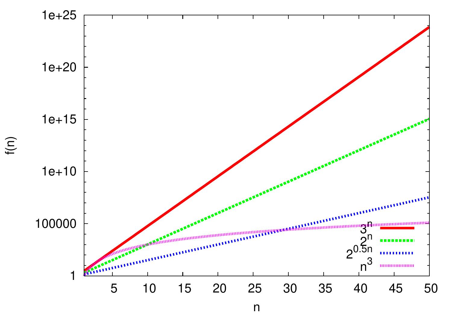
The plot below shows some functions. Please observe the logarithmic scale on the $ f(n) $-axis: compared to the linear scale, it allows easier visual comparison of different functions with orders of magnitude difference in values.

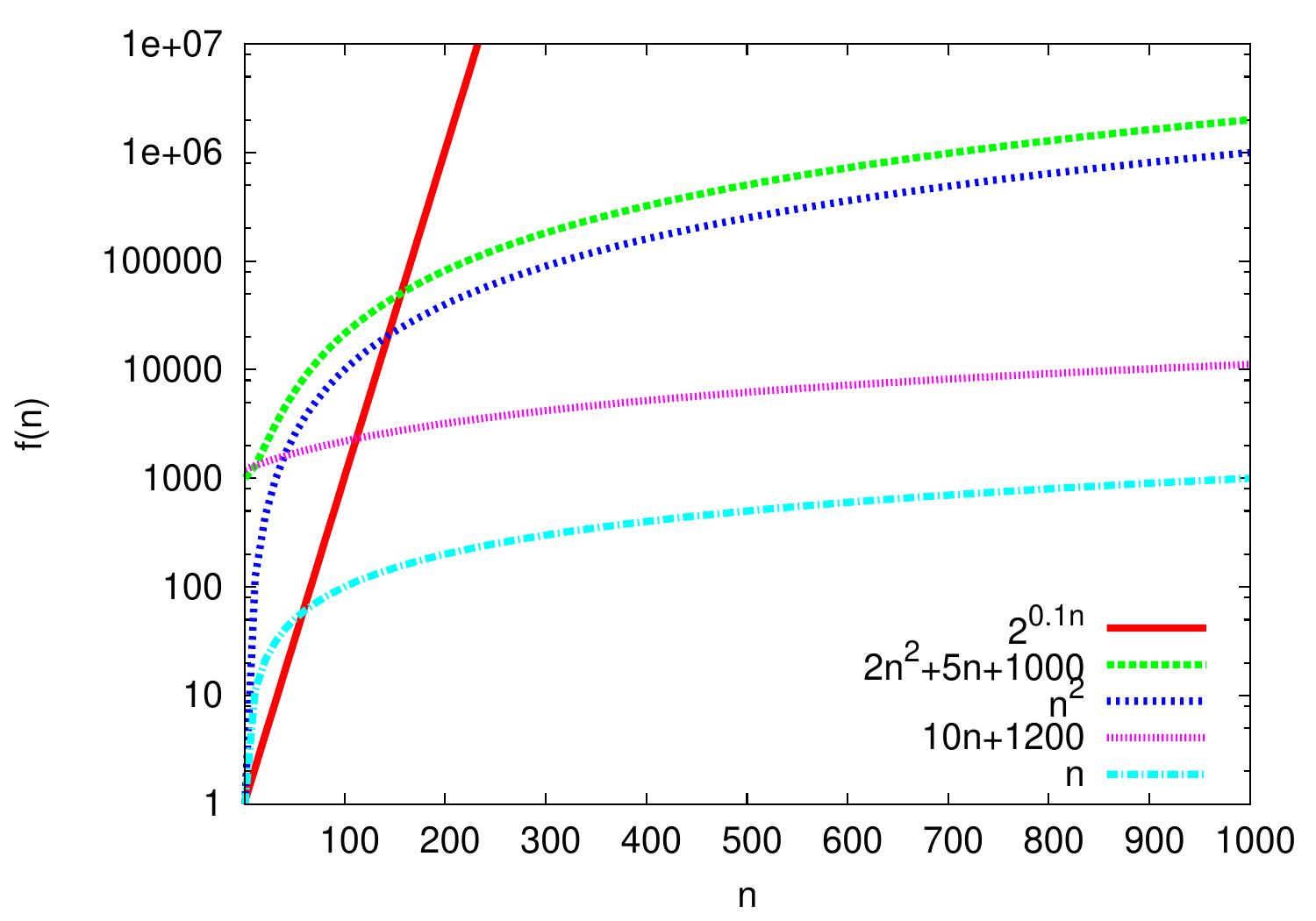
In the plot we easily see that the functions $ n $ and $ 10n+1200 $ seem to behave similarly: for larger values of $ n $, the difference between their lines seems to keep constant. As the $ y $-axis is logarithmic, this means that the value of $ 10n+1200 $ seems to be a constant factor larger than that of $ n $. Thus the functions seem to grow in the same rate. And indeed:

$ n = \Oh{10n+1200} $ as $ n \le 1(10n+1200) $ for all $ n \ge 1 $, and
$ 10n+1200 = \Oh{n} $ as $ 10n+1200 \le 12n $ for all $ n \ge 600 $.

Thus $ 10n+1200 = \Theta(n) $ and the functions do grow at the same rate.

Similarly, $ 2n^2++5n+1000 = \Theta(n^2) $ and thus $ n^2+5n+1000 $ and $ n^2 $ grow at the same rate. On the other hand, $ n = \Oh{n^2} $ but $ n^2 \neq \Oh{n} $. In fact, $ n = o(n^2) $ and $ n $ grows slower than $ n^2 $. One can see this in the plot as well: the difference between the lines $ n $ and $ n^2 $ keeps increasing.

Similarly, $ n = \Oh{2^{0.1n}} $ but $ 2^{0.1n} \neq \Oh{n} $. Indeed, $ 2^{0.1n} = \omega(n) $ and $ 2^{0.1n} $ grows faster than $ n $. So although for very small values of $ n $ it holds that $ 2^{0.1n} < n $, the growth rate of $ 2^{0.1} $ is much higher than that of $ n $.

Some typical function families encountered in practise:

$ \Oh{1} $ — constant
$ \Oh{\log n} $ — logarithmic
$ \Oh{n} $ — linear
$ \Oh{n \log n} $ — linearithmic, “n log n”. Observe that $ \Oh{\log n!} = \Oh{n \log n} $.
$ \Oh{n^2} $ — quadratic
$ \Oh{n^3} $ — cubic
$ \Oh{n^k} $ — polynomial, $ k \ge 0 $
$ \Oh{c^n} $ — exponential, $ c > 1 $
$ \Oh{n!} $ — factorial

Constant, logarithmic, linear, linearithmic, quadratic, and cubic functions are all polynomial functions. We use base-2 logarithms unless otherwise stated but, in the context of O-notation, this is usually not relevant as $ \log_c n = \frac{\log_2 n}{\log_2 c} $ for any $ c > 1 $ and $ \log_2 c $ is a constant when $ c $ is a constant.

Example: Additive constants

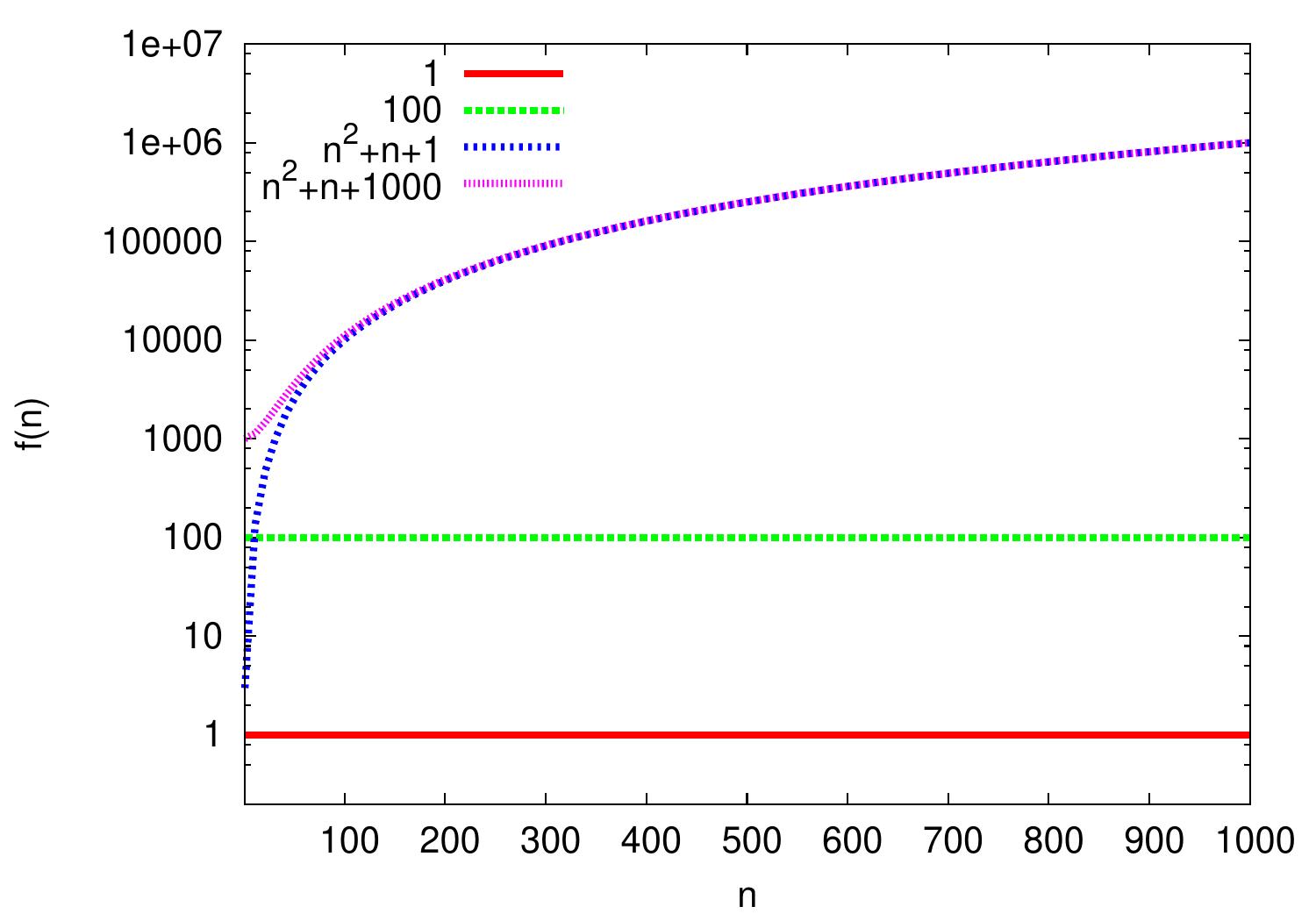
Additive constants are irrelevant in Big O notation as we consider asymptotic growth rate of functions.

For instance, $ 100 = \Oh{1} $ as for all $ n \ge n_0 = 1 $, $ 100 \le 100 \times 1 $.

Similarly, $ n^2 + n + 1000 = \Oh{n^2+n+1} $ because $ n^2 + n + 1000 \le 1000(n^2+n+1) $ for all $ n \ge n_0 = 1 $

Example: Polynomials

In polynomials, the largest degree dominates.

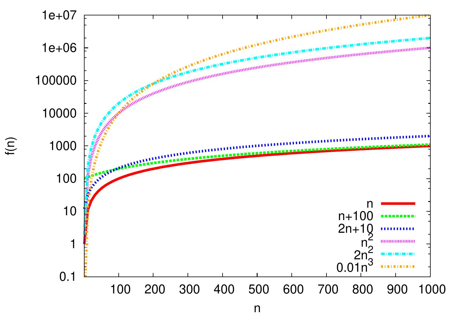
$ 2n+10 = \Oh{n} $ as $ \frac{2n+10}{n}=2+\frac{10}{n} \le 3 $ and thus $ 2n+10 \le 3n $ for all $ n \ge n_0 = 10 $.
$ n^2 = \Oh{0.01n^3} $ because $ \frac{n^2}{0.01n^3} = \frac{100}{n} \le 1 $ and thus $ n^2 \le 0.01n^3 $ for all $ n \ge n_0 = 100 $.
$ 0.01n^3 \neq \Oh{n^2} $ because for all $ n_0, c > 0 $, we can choose $ n > \max\{100c,n_0\} $ and then $ 0.01n^3 > cn^2 $.

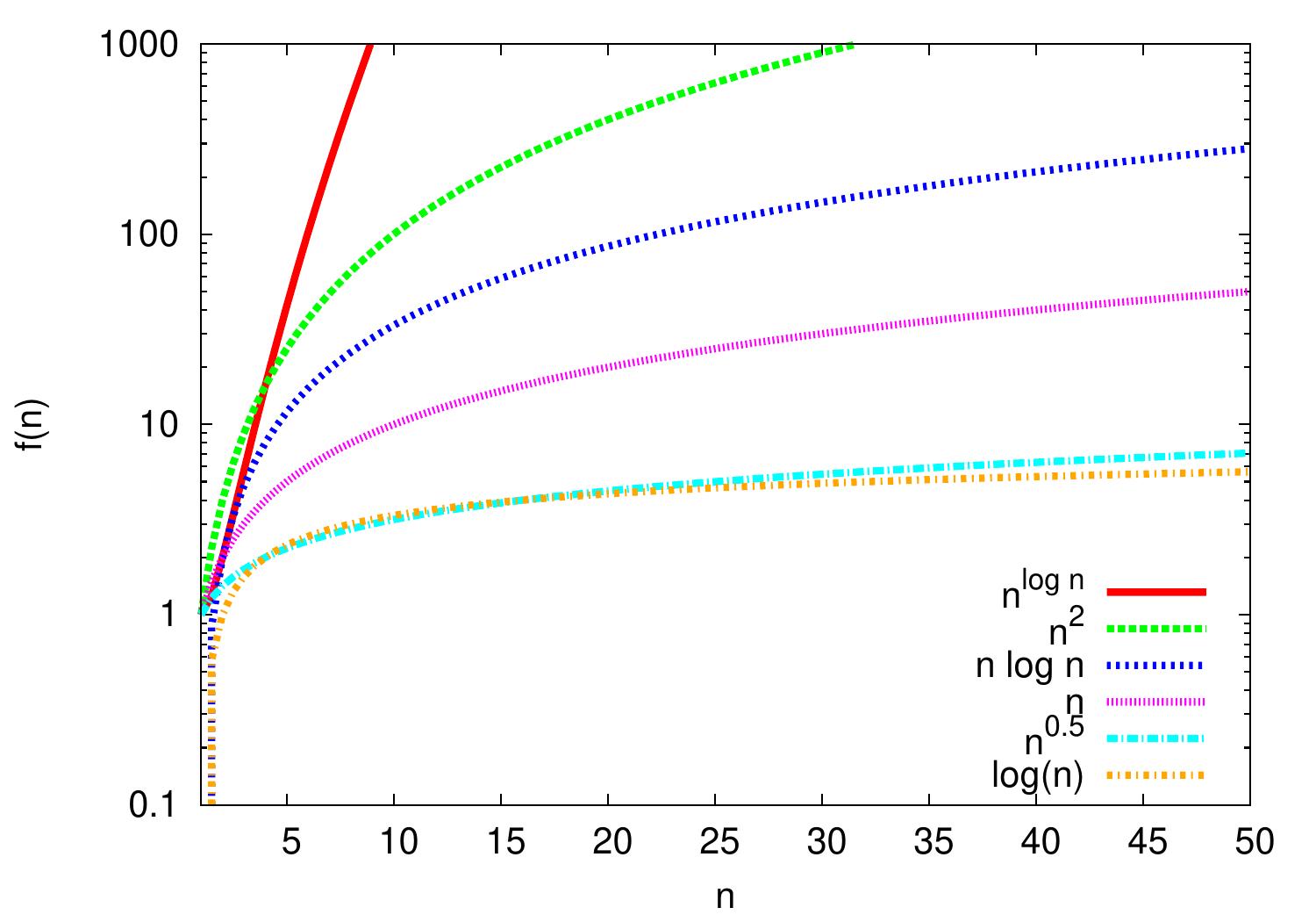
Example: Logarithms

The logarithmic function $ \log n $ grows rather slow but faster than any constant. It grows slower than any polynomial $ n^k $, where $ k > 0 $ is a constant.

$ \log n = \Oh{n} $ but $ n \neq \Oh{\log{n}} $
$ \log n = \Oh{\sqrt{n}} $ but $ \sqrt{n} \neq \Oh{\log{n}} $
$ n \log n = \Oh{n^2} $ but $ n^2 \neq \Oh{n \log{n}} $
$ n^2 = \Oh{n^{\log n}} $ but $ n^{\log n} \neq \Oh{n^2} $

Example: Exponential functions

Exponential functions grow faster than polynomials. That is, $ c^n $ grows faster than $ n^k $, where $ c > 1 $ and $ k > 0 $ are constants. The base matters: for instance, $ 2^n = \Oh{3^n} $ but $ 3^n \neq \Oh{2^n} $. Constant factors in the exponent also matter because, for instance, $ 2^{cn} = (2^c)^n $ for a constant $ c > 0 $. But notices that in running-time analysis of algorithms, functions of the form $ 2^{n^k} $, where $ k $ is a constant, are also commonly called exponential functions.

Running times of algorithms¶

Definition

The worst-case running time of a program/algorithm is $ \Oh{f(n)} $ if $ g(n) = \Oh{f(n)} $, where the function $ g(n) $ is obtained by taking, for each $ n $, the longest running time of any input of size $ n $.

When we say “a program/algorithm runs in time $ \Oh{f(n)} $”, we usually mean that its worst-case running time is $ \Oh{f(n)} $. Similarly for the $ \Theta $ and $ \Omega $ notations. One may also consider

the best-case running time obtained by taking the smallest running times for each $ n $, and
the average-case running time by taking the mean of the running times for each $ n $ over some set of inputs (usually all valid inputs).

Example: Linear search

Consider the simple linear search algorithm with the following input/output specification:

Input: an unordered array $ A $ of $ n $ elements and an element $ e $
Output: does $ e $ appear in $ A $?

The algorithm is:

// Search for the element \( e \) in the array \( A \)
linear-search(\( A \), \( e \)):
  for \( i \in [1..\ALengthOf{A}] \):
    if \( A[i] \Eq e \): return true
  return false
 

Assume that array accesses and element comparisons are constant time operations.

The worst-case running time is $ \Theta(n) $. This occurs when the element may not be included in the array. In this case, the whole for-loop is executed. In each loop body iteration, some constant amount $ c $ of time is spent in its instructions (array access, comparison, loop index increase). At the end, “false” is returned in some constant time $ d $. Thus the running time is $ \Theta(nc+d)=\Theta(n) $.
The best-case running time is $ \Theta(1) $ as $ e $ can be the first element in the array. In this case, only one array access and one comparison operation are performed.

Example: Straightforward multiplication of $ n \times n $ square matrices

Consider two $ n \times n $ matrices $ (a_{ij}) $ and $ (b_{ij}) $ with $ 1 \le i,j \le n $. The method * in the Scala code below computes the $ n \times n $ product matrix $$c_{ij} = \sum_{k=1}^n a_{ik} b_{kj}$$

class Matrix(val n: Int) {
  require(n > 0, "n must be positive")
  val entries = new Array[Double](n * n)
  /** Access elements by writing m(i,j) */
  def apply(row: Int, column: Int) = {
    entries(row * n + column)
  }
  /** Set elements by writing m(i,j) = v */
  def update(row:Int, col:Int, val:Double) {
    entries(row * n + col) = val
  }
  /** Returns the product of this and that */
  def *(that: Matrix): Matrix = {
    require(n == that.n)
    val result = new Matrix(n)
    for (row <- 0 until n; column <- 0 until n) {
      var v = 0.0
      for (i <- 0 until n)
        v += this(row, i) * that(i, column)
      result(row, column) = v
    }
    result
  }
}

Let’s analyze the asymptotic running time of the multiplication method *.

Initializing the result matrix takes $ \Theta(n^2) $ steps as the $ n \times n $ matrix is allocated and initialized to $ 0 $s.
The outer loop iterates row from $ 0 $ to $ n-1 $.
The middle loop iterates column from $ 0 $ to $ n-1 $.
The inner loop iterates i from $ 0 $ to $ n-1 $.
Inside the inner loop, the multiplication and array accesses are constant time operations.
Because of the above four items, the for-loops part takes $ \Theta(n^3) $ time.

To sum up, the running time of the * method is $ \Theta(n^2+n^3) = \Theta(n^3) $.

Recursion and Recurrences¶

For recursive programs, it can be more difficult to analyze the asymptotic running time directly from the (pseudo)code.

Example: Binary search (recursive version)

From the CS-A1120 Programming 2 course, recall the binary search algorithm for searching an element in a sorted array, implemented below in Scala.

def binarySearch[T <% Ordered[T]](arr: Array[T], e: T): Boolean = {
  def inner(lo: Int, hi: Int): Boolean = {
    if(lo <= hi) {
      val mid = lo + ((hi - lo) / 2)
      val cmp = e compare arr(mid)
      if(cmp == 0) true                 // e == arr(mid)
      else if(cmp < 0) inner(lo, mid-1) // e < arr(mid)
      else inner(mid+1, hi)             // e > arr(mid)
    } else
      false
  }
  inner(0, arr.length-1)
}

But in fact analyzing corresponding iterative versions may not be easier either. For instance, consider the iterative version of the binary search algorithm below.

def binarySearch[T <% Ordered[T]](arr: Array[T], v: T): Boolean = {
  var lo = 0
  var hi = arr.length - 1
  while(lo <= hi) {
    val mid = lo + ((hi - lo) / 2)
    val cmp = v compare arr(mid)
    if(cmp == 0) return true;    // v == arr(mid)
    else if(cmp < 0) hi = mid-1  // v < arr(mid)
    else lo = mid+1              // v > arr(mid)
  }
  return false
}

To obtain an asymptotic running time estimate for recursive programs, one can try to formulate the running time (or some other measure) $ T(n) $ on inputs of size $ n $ as a recurrence equation of form $$T(n) = …$$ where

$ n $ is some parameter usually depending on the (current) input size, and
the right hand side recursively depends on the running time(s) $ T(n’) $ of some smaller values $ n’ $ and some other terms.

In addition, the base cases, usually $ T(0) $ or $ T(1) $, not depending on other $ T(n’) $ need to be given. One then solves the equation somehow. Note that $ T(n) $ is not the value that the function computes but the number of steps taken when running the algorithm on an input of size $ n $.

Example: Recurrence for binary search

Consider again the recursive binary search program below.

def binarySearch[T <% Ordered[T]](arr: Array[T], e: T): Boolean = {
  def inner(lo: Int, hi: Int): Boolean = {
    if(lo <= hi) {
      val mid = lo + ((hi - lo) / 2)
      val cmp = e compare arr(mid)
      if(cmp == 0) true                 // e == arr(mid)
      else if(cmp < 0) inner(lo, mid-1) // e < arr(mid)
      else inner(mid+1, hi)             // e > arr(mid)
    } else
      false
  }
  inner(0, arr.length-1)
}

The recursive part considers sub-arrays of size $ n $, where $ n $ equals to hi - lo + 1 in our implementation above.

If $ n \le 0 $, the recursion terminates with “false”.
If $ n \ge 1 $, a comparison is made and
- the search either terminates with “true” (the element was found) or
- the same recursive function is called with a sub-array of size at most $ \lfloor n/2 \rfloor $.

Assuming that array accesses and element comparisons are constant-time operations, we thus get the recurrence equations $$T(0) = d \text{ and } T(n) = c + T(\lfloor n/2 \rfloor)$$ where $ d $ and $ c $ are some constants capturing the number of operations taken to compare the bound, comparison etc. Here $ T(n) $ is a worst-case upper bound for the running time (number of instructions executed) on arrays with $ n $ elements as we have omitted the early termination case when the element is found but assume that the recursion always runs until the base case of arrays of size 0.

Let’s solve the recurrence equations $$T(0) = d \text{ and } T(n) = c + T(\lfloor n/2 \rfloor)$$ In this case, we obtain an upper bound by considering inputs of length $ n = 2^k $ for some non-negative integer $ k $. Now $$T(2^k) = c + T(2^{k-1}) = c + (c + T(2^{k-2})) = … = k c + T(2^{0}) = c (k+1) + d$$ As $ n = 2^k $ implying $ k = \Lg n $, and $ c $ and $ d $ are constants, we get $$T(n) = T(2^k) = c k + c + d = c \Lg n + c + d = \Oh{\Lg n}$$

When $ n $ is not a power of two, $ T(n) \le T(2^{\lceil \Lg n\rceil}) = c \lceil \Lg n\rceil + 2c + d = \Oh{\Lg n} $ as $ T(n) $ is monotonic.

When using the $ \BigOh $-notation, constants can be usually eliminated already in the beginning by replacing them with $ 1 $. In our binary search example, the recurrence is thus $$T(0) = 1 \text{ and } T(n) = 1 + T(\lfloor n/2 \rfloor)$$ Solving this gives again $ T(n) = \Oh{\Lg n} $. Sometimes one also writes $$T(0) = \Oh{1} \text{ and } T(n) = \Oh{1} + T(\lfloor n/2 \rfloor).$$

In addition to the number of instructions taken, we may sometimes be interested in some other aspects of the algorithm. For instance, if we know that comparisons are very expensive, we may analyze how many of them are taken in a search or sorting algorithm.

Example

For binary search, an asymptotic upper bound for the number of comparisons made on an input of elements $ n $ can be obtained again by the recurrence $$T(0) = T(1) = 1 \text{ and } T(n) = T(\lfloor n/2 \rfloor) + 1$$ and thus $ T(n) = \Oh{\Lg n} $.

We’ll see slightly more complex recurrences later when analyzing sorting algorithms.

Example: The subset sum problem

Consider the subset sum problem:

Given a set $ S = \Set{v_1,…,v_n} $ of integers and a target integer $ t $. Is there a subset $ S’ $ of $ S $ such that $ \sum_{v \in S’}v = t $?

Below is a (very simple) recursive Scala program solving it:

def subsetsum(s : List[Int], t : Int) : Option[List[Int]] = {
  if(t == 0) return Some(Nil)
  if(s.isEmpty) return None
  val solNotIncluded = subsetsum(s.tail, t)
  if(solNotIncluded.nonEmpty) return solNotIncluded
  val solIncluded = subsetsum(s.tail, t-s.head)
  if(solIncluded.nonEmpty) return Some(s.head :: solIncluded.get)
  return None
}

Let’s form a recurrence for the running time of the recursive program with the parameter $ n $ being the size of the set. In the worst-case scenario, there is no solution and the recursion terminates only when the set is empty. In each call, the program makes some constant-time tests etc and then two recursive calls with a set that has one element removed. Thus we get the recurrence $$T(0) = 1 \text{ and } T(n) = 1 + T(n-1) + T(n-1) = 1 + 2T(n-1)$$ Expanding the recurrence, we get \begin{eqnarray*} T(n) &=& 1 + 2T(n-1)\\ &=& 1 + 2(1+2T(n-2))\\ &=& 1 + 2 + 4(1 + 2T(n-3))\\ &=& … \\ &=& \sum_{i=0}^n 2^i\\ &=& 2^{n+1}-1 \\ &=& \Theta(2^{n}) \end{eqnarray*} Thus the algorithm takes exponential time in the worst case.

In the (very rare) best case, the target equals to $ 0 $ and the program takes a constant time to complete.