Experimental analysis¶

The O-notation described earlier disregards constant factors. In practice, however, constant factors in running times and other resource usages do matter. In addition to mathematical analysis, we may thus perform experimental performance analysis. For instance, we may

take implementations of two algorithms that perform the same task,
run these on the same input set, and
compare their running times.

Similarly, we may

instrument the code, for instance, to count all the comparison operators made and then run the algorithm on various inputs to see how many comparisons are made on average or in the worst case, or
use some profiling tool (such as valgrind for C/C++/binary programs) to find out numbers of cache misses etc.

Example: Square matrix multiplication

Let’s compare the performance of some \( n \times n \) matrix multiplication implementations:

Scala naive: the code in Section Running times of algorithms
C++ naive: the same in C++
Scala transpose: transpose the other matrix for better cache behavior
Scala transpose parallel: the previous but use 8 threads of a 3.20GHz Intel Xeon(R) E31230 CPU
cuBLAS (GPU): use NVIDIA Quadro 2000 (a medium range graphics processing unit) and a well-designed implementation in the NVIDIA cuBLAS library (version 7.5)

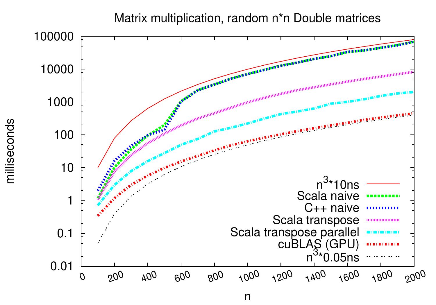
We see that the implementations scale similarly but on \( 2000 \times 2000 \) matrices (and on this particular machine), the running times drop from the \( 68\mathrm{s} \) of the naive algorithm to \( 0.45\mathrm{s} \) of the GPU algorithm.

Simple running time measurement in Scala¶

As seen in the CS-A1120 Programming 2 course, we can measure running times of functions quite easily.

import java.lang.management.{ManagementFactory, ThreadMXBean}
package object timer {
  val bean: ThreadMXBean = ManagementFactory.getThreadMXBean()
  def getCpuTime = if(bean.isCurrentThreadCpuTimeSupported())
    bean.getCurrentThreadCpuTime() else 0
  def measureCpuTime[T](f: => T): (T, Double) = {
    val start = getCpuTime
    val r = f
    val end = getCpuTime
    (r, (end - start) / 1000000000.0)
  }
  def measureWallClockTime[T](f: => T): (T, Double) = {
    val start = System.nanoTime
    val r = f
    val end = System.nanoTime
    (r, (end - start) / 1000000000.0)
  }
}

Observe that wall clock times (the function measureWallClockTime) should be used when measuring running times of parallel programs. This is because the method getCurrentThreadCpuTime used in measureCpuTime measures the CPU time of only one thread.

Unfortunately, things are not always that simple. Let’s run the following code which sorts twenty arrays of 10000 integers:

import timer._
val a = new Array[Int](10000)
val rand = new scala.util.Random()
val times = scala.collection.mutable.ArrayBuffer[Double]()
for(test <- 0 until 20) {
  for(i <- 0 until a.length) a(i) = rand.nextInt
  val (dummy, t) = measureCpuTime { a.sorted }
  times += t
}
println(times.mkString(", "))

An output of the program:

0.024590893, 0.010173347, 0.005155264, 0.003917635, 0.002668954, 0.002594947, 0.002807369, 0.002570412, 0.004068068, 0.006141965, 0.005393813, 0.005688233, 0.005168036, 0.005198876, 0.005008517, 0.004631029, 0.002407551, 0.001865849, 0.001878646, 0.002058858

The program measures the same code on similar inputs but the running times improve significantly after some repetitions. Why is this happening? The above behaviour can be explained as follows.

A Scala program is first compiled into Java bytecode.
The resulting Java bytecode is executed in a Java virtual machine (JVM).
The execution may start in interpreted mode.
After while, some parts of the program can then be just-in-time compiled to native machine code during the execution of the program.
The compiled code may then be globally optimized during the execution.
In addition, garbage collection may happen during the execution.

As a consequence, when measuring running times of programs with shortish running times, one should be careful when interpreting the results. But for programs with larger running times this is usually not so big problem.

As we saw, reliably benchmarking programs written in interpreted and virtual machine based languages (such as Java and Scala) can be challenging, especially if the running times are small. In this course, we’ll sometimes use the ScalaMeter tool for performance analysis. It tries to take the JVM-related issues into account by, among other things, “warming up” the virtual machine and using statistical analysis techniques. See, for instance, the documentation of the tool and the article

Georges et al: Statistically rigorous java performance evaluation, Proc. OOPSLA 2007, pp. 57-76.