Hashing and hash tables¶

In a sense, hash tables extend the idea of Direct-access tables to very large, or even infinite, key universes $ U $. Note that at any given time, only a finite subset $ K \subseteq U $ of the possible keys are stored in a table. The main idea is to

have a hash table (an array) of $ m $ entries, and
then use a hash function $$h : U \to \Set{0,1,…,m-1}$$ to map each key to an index in in the table. The value $ h(k) $ is called the hash value of the key $ k $.

In the ideal case, each key should map to a different index but in general this is difficult to obtain efficiently (and impossible when $ \Card{K} > m $). Thus there will be collisions when two keys should be put in the same table index.

Example

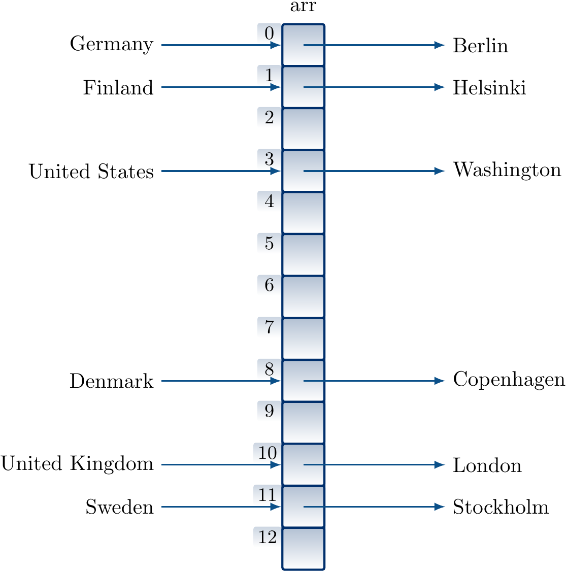
Assume a hash table with $ m = 13 $ entries and a hash function for strings implemented in Scala 2.11.8 with

def h(s: String) = math.abs(s.hashCode) % 13

where We’ll later see how hashCode of a string is computed. Many strings map to different indices and the basic idea described above works “as is”:

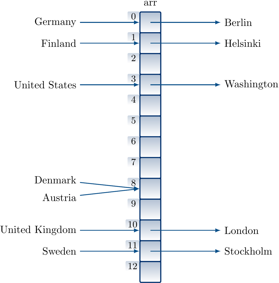
However, some strings map to the same index causing collisions. As an example, with the above hash function “Denmark” and “Austria” are mapped to the same index.

How probable are collisions? Suppose a hash function $ h $ under the simple uniform hashing assumption:

Any key is equally likely to hash to a value in $ \Set{0,1,…,m-1} $ independently of the other keys.

Under the assumption, the number of randomly drawn keys such that at least one collision is produced with probability $ p $ is $$\approx \sqrt{2 m \ln\left(\frac{1}{1-p}\right)}$$ As an example, for a hash table with $ m = 1\,000\,000 $ entries, we only need to insert only $ 1178 $ random keys to produce at least one collision with probability of 0.5. As a consequence, collisions become rather likely quite soon! A special case of this is called the birthday paradox: there are 365 days in a year but if we have 23 randomly selected people in the same room, the probability that there are two people having the same birthday is at least 0.5, assuming that the birthdays of people in general are evenly distributed over a year.

In order to handle the inevitable collisions, we need a collision resolution scheme. In the following, we’ll see two schemes, namely

chaining, and
open hashing with some variants.

First, we need an additional definition:

Definition: Load factor

The load factor of a hash table with $ m $ entries and $ n $ keys stored in it is $ \alpha = n/m $.

Chaining¶

Chaining is a collision resolution method and it is also called separate chaining and open hashing in some texts. The idea in chaining is as follows: each entry in the hash table starts a linked list and the key/value-pairs are stored in the list. After finding the index $ h(k) $, and thus the correct list for a key $ k $, the rest is as with mutable linked lists:

search: traverse the list to see if the key is stored in an entry.
insert: traverse the list and insert a new entry at the end of the list if the key was not found. If the key was found, replace the old value in the list entry with the new one.
remove: traverse the list and remove the list entry if the key was found.

Example: Collision handling with chaining

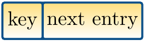
The entries in the linked lists are drawn as

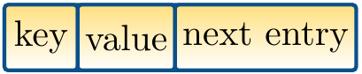
where

key is the key (or a reference to it in the case of a non-primitive key type),
value is the value (or a reference to it), and
next entry is a reference to the next entry in the list (null if the current entry is the last one).

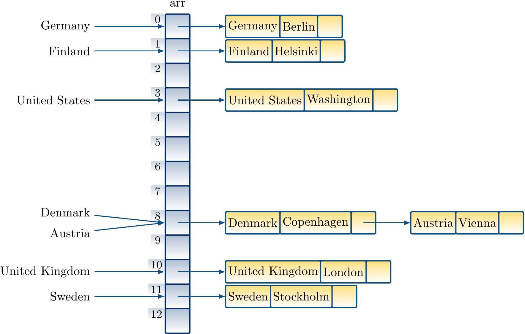
The collision between Austria and Denmark is now resolved by inserting Austria in the list after Denmark:

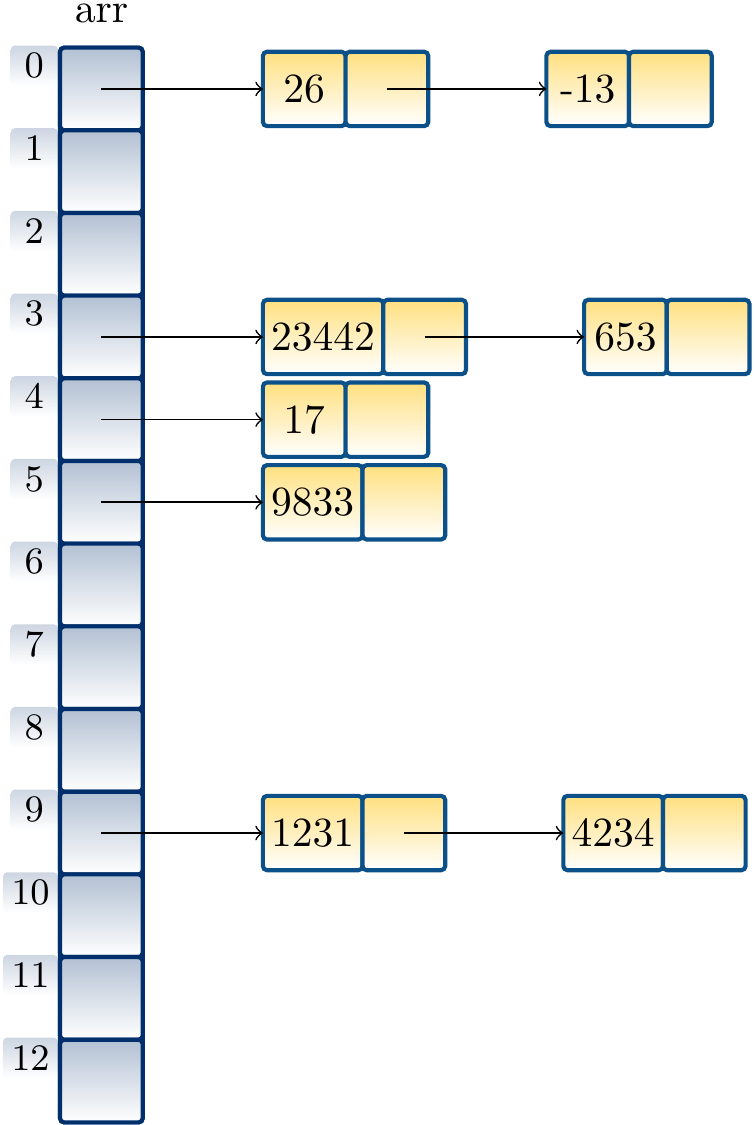
Example: Implementing sets with hashing and chaining

If we are not interested in maps but in sets, we just drop the value field and use entries of the following form in the lists:

Inserting the numbers 1231, 9833, 23442, 26, 17, 4234, 653 and -13 in a “hash set” of integers with the hash function $ h(k) = k \bmod m $ produces the following hash table when $ m = 13 $:

Example: Unordered sets in C++11

The unordered set data type of C++11 is implemented with open hashing in the GNU ISO C++ library version 4.6. The library also implements the hash functions and key equality comparators for the basic types and we can thus write the following:

#include <iostream>
#include <unordered_set>
int main ()
{
  // A set of small prime numbers
  std::unordered_set<int> myset = {3,5,7,11,13,17,19,23,29};
  myset.erase(13);                         // erasing by key
  myset.erase(myset.begin());              // erasing by iterator
  std::cout << "myset contains:";
  for (const int& x: myset) std::cout << " " << x;
  std::cout << std::endl;
  return 0;
}

One possible output of the program is shown below. Note that the elements are not ordered and the line myset.erase(myset.begin()) erasing the “first” element in the set did not erase 3 but 23 as with the current keys and the applied hash function, 23 happened to be the “first” key in the table.

myset contains: 19 17 11 29 7 5 3

Similar hashing-based classes are also available in C++11 for unordered multisets, maps, and multimaps.

Analysis¶

For the analysis, assume that computing the hash value $ h(k) $ for each key takes constant $ \Oh{1} $ time. Suppose that we have inserted $ n $ keys in a hash table with $ m $ entries. Under the simple uniform hashing assumption, the expected number of keys in the linked list at an index $ i $ is $ \frac{n}{m} $. The cost of searching for a key in the hash table is thus $ \Oh{1 + \frac{n}{m}} $, equalling to $ \Oh{1+\alpha} $, on average in both cases when the key is not found and when it is found in the table. When $ n $ is proportional to $ m $, meaning that $ n \le c m $ for some constant $ c $ and thus $ \alpha \le c $, then searching takes time $ \Oh{1+\frac{c m}{m}} = \Oh{1} $ on average. If the insert and remove operations first search whether the key is in the table, then they also take time $ \Oh{1} $ on average if $ n \le c m $ for some constant $ c $. Thus

inserting, searching, and removing keys can be done in constant time on average if the load factor of the hash table is below come fixed constant.

The worst-case behaviour occurs when all the keys hash to the same index:

the hash table effectively reduces to a linked list, and
inserting, searching, and removing keys require $ \Theta(n) $ time.

Therefore, good design of hash functions is important.

Rehashing¶

How large a hash table should we allocate in the beginning if/when we do not know how many keys will be seen in the future? Or, what should we do when the load factor grows too large? The answer is rehashing: start with a smallish hash table and then grow its size when the load factor rises above certain fixed threshold. When the hash table is resized, all the keys (or key/value pairs in maps) must be reinserted to it as their indices in the table are probably changed. This is why the method is called “rehashing”.

What is a good constant upper bound value for the load factor for triggering rehashing? There is no single best answer; the GNU ISO C++ library version 4.6 triggers rehashing when the load factor is above 1.0 and then doubles the number of entries in the hash table.

Open addressing¶

Open addressing is another collision resolution scheme. In some texts, it is also called closed hashing. The main idea in open addressing is to always use an array large enough to hold all the inserted keys. Thus each array index

stores one key/value pair (or simply the key if we are implementing a set instead of a map), or
is null (or some other special symbol) when it is free.

Thus the load factor is always at most 1.0 in open addressing. When a collision occurs during an insert, we probe another index in the table until a free one is found. Similarly, when searching for a key, one probes indices until the key is found or an empty slot is encountered.

For probing, we need to define which index is tried next. To do this, we define a hash function to be of the form $$h: U \times \Set{0,1,…,m-1} \to \Set{0,1,…m-1}$$ where the second argument is the probe number. For each key $ k $, the probe sequence is thus $$h(k,0),h(k,1),…,h(k,m-1).$$ To ensure that every index in the table is probed at some point, the probe sequence must be a permutation of $ \Set{0,1,…,m-1} $ for every key $ k $.

Linear probing¶

Linear probing is the simplest way to define probe sequences. Suppose that we already have a “real” hash function $ h’: U \to \Set{0,1,…,m-1} $, which usually is the hash function provided by the class or user (for instance, the function implemented in a hashCode method in Scala). Now define the probe sequence hash function as $$h(k,i) = (h’(k)+i) \bmod m$$ Clearly, the probe sequence $ h(k,0),h(k,1),…,h(k,m-1) $ is a permutation of $ \Set{0,1,…,m-1} $.

Example: Collision resolution with linear probing

The entries in the table are drawn as

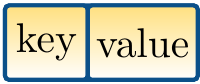
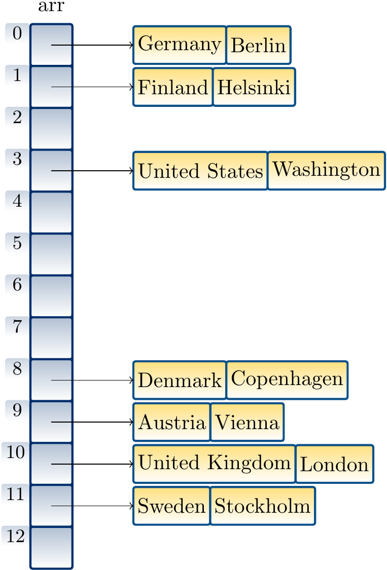
where again key is the key (or a reference to it in case of a non-primitive type), and value is the value (or a reference to it). Inserting the key/value pairs

Finland ↦ Helsinki
United States ↦ Washington
United Kingdom ↦ London
Denmark ↦ Copenhagen
Austria ↦ Vienna
Sweden ↦ Stockholm

in a table of size 13 in this order by using our ealier hash function and linear probing gives the hash table below. When inserting the mapping “Austria ↦ Vienna”, we observe that the index 8 is already taken by Denmark, probe the next index 9, see that it is free, and insert the key/value pair there.

Example: Sets with hashing and linear probing

When implementing sets instead of maps, the table entries consist of the key values (or references to them) only.

For instance, inserting the numbers 1231, 9833, 23442, 26, 17, 4234, 653 and -13 in a hash table of integers with $ m = 13 $ by using the auxiliary hash function $ h’(k) = k $ produces the hash table shown below.

$ 1231 $ is inserted to $ h(1231,0) = (1231+0) \bmod 13 = 9 $
$ 9833 $ is inserted to $ h(9833,0) = (9833+0) \bmod 13 = 5 $
$ 23442 $ is inserted to $ h(23442,0) = (23442+0) \bmod 13 = 3 $
$ 26 $ is inserted to $ h(26,0) = (26+0) \bmod 13 = 0 $
$ 17 $ is inserted to $ h(17,0) = (17+0) \bmod 13 = 4 $
as $ h(4234,0) = (4234+0) \bmod 13 = 9 $ is occupied, the next index $ h(4234,1) = (4234+1) \bmod 13 = 10 $ is probed, found free, and $ 4234 $ is inserted there
as $ h(653,0) = (653+0) \bmod 13 = 3 $ is occupied, the next indices $ h(653,1) = 4 $ and $ h(653,2) = 5 $ are probed and found occupied, and finally $ 653 $ is inserted to $ h(653,3) = 6 $
as $ h(-13,0) = 0 $ is occupied, $ -13 $ is inserted to the next free index $ h(-13,1) = 1 $

In the following examples, for representational simplicity only, we only consider “hash sets” for integers — generalization to maps over arbitrary key and value types is straightforward.

Linear probing suffers from the problem called primary clustering:

an empty slot preceded by $ i $ occupied slots gets filled with probability $ (i+1)/m $ instead of $ 1/m $, and
thus occupied slots start to cluster.

Example

Suppose that $ h’(k) = k $ for integer-valued keys and $ m = 17 $. Inserting the values $ 1 $, $ 50 $, $ 2 $, $ 20 $, $ 38 $, $ 35 $ in this order with linear probing produces the hash table

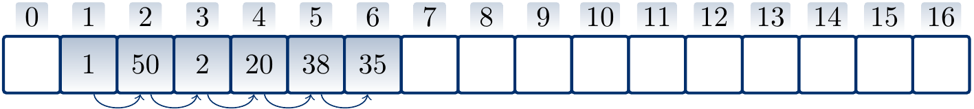
where the arrows show the probe sequence for the key $ 35 $. Note that only $ 1 $, $ 50 $, and $ 35 $ of the above keys hash to the same value.

Quadratic probing¶

Quadratic probing eliminates the primary clustering problem by using more complex probing sequences. Define the probing sequence hash function $$h(k,i) = (h’(k) + c_1 i + c_2 i^2) \bmod m$$ where $ c_1 $ and $ c_2 $ are some positive constants and $ h’ : K \to \Set{0,1,…M} $ for $ M \ge m $ is again the “real” hash function. To make the probe sequence a permutation of $ \Set{0,1,…,m-1} $, the values $ c_1 $, $ c_2 $, and $ m $ must be constrained.

Example: Bad parameters

Assume that $ m = 11 $ (i.e., a prime) and $$h(k, i) = (h’(k) + i + i^2) \bmod m.$$ If $ h’(k) = 0 $, then the probe sequence is $ 0, 2, 6, 1, 9, 8, 9, 1, 6, 2, 0 $. This is not a permutation of $ \Set{0,1,…,10} $ but probes only 6 of 11 possible slots. Thus if the load factor is high, this probe sequence may not find any free slots.

Example

Assume that $ m $ is a power of two. In this case, it can be proven that $$h(k, i) = (h’(k) + \frac{i(i+1)}{2}) \bmod m = (h’(k)+ 0.5i + 0.5i^2) \bmod m$$ produces probe sequencies that are permutations of $ \Set{0,1,….,m} $. For instance, if $ m = 2^3 = 8 $ and $ h’(k) = 0 $, then the probe sequence is $ 0, 1, 3, 6, 2, 7, 5, 4 $.

Example

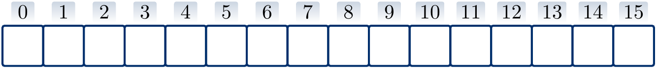
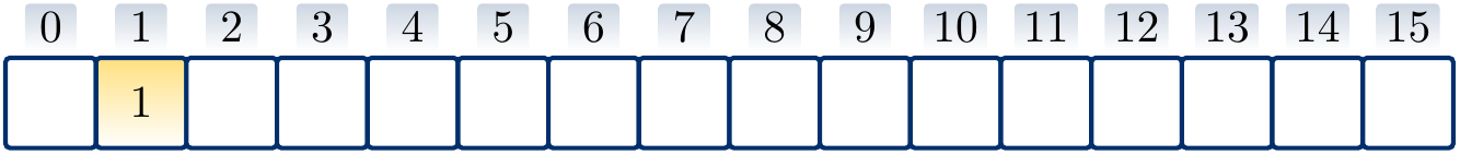
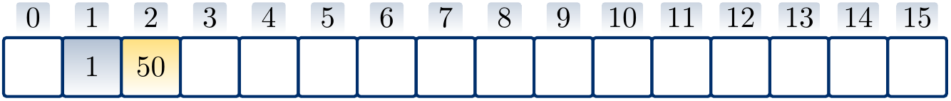
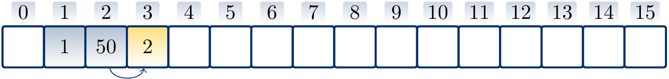
Suppose that $ h’(k) = k $ for integer-valued keys and $ m = 16 $. Let us insert the values $ 1 $, $ 50 $, $ 2 $, $ 20 $, $ 38 $, $ 35 $ in this order with quadratic probing hash function $ h(k) = (h’(k) + \frac{i(i+1)}{2}) \bmod m $ to the empty hash table. Again, the arrows below the table show the applied probe sequences.

The situation in the beginning.
Inserting $ 1 $.
Inserting $ 50 $.
Inserting $ 2 $.
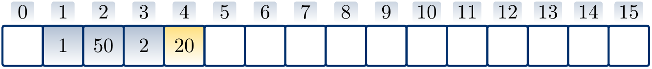
Inserting $ 20 $.
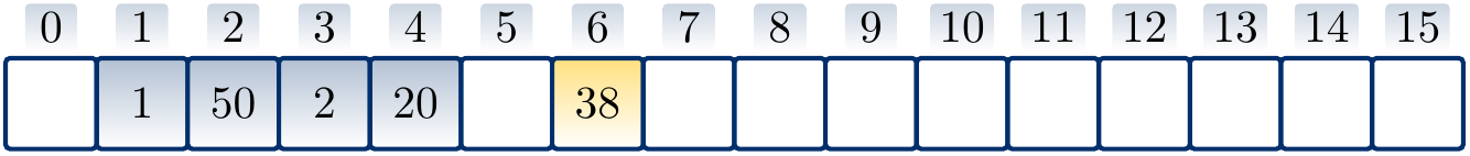
Inserting $ 38 $.
Inserting $ 35 $.

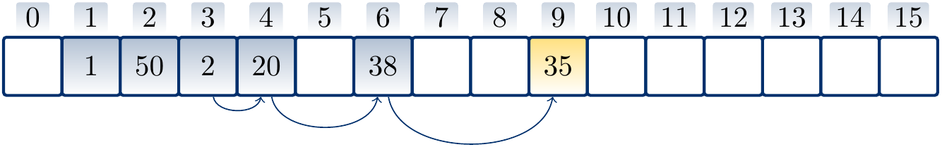
Unlike linear probing, quadratic probing does not suffer from primary clustering. But two keys $ k_1 $ and $ k_2 $ with the same hash value $ h’(k_1) = h’(k_2) $ have the same probe sequence. This, admittedly less severe, problem with quadratic probing is called secondary clustering. Another inoptimality of linear and quadratic probings is the following:

For hash tables of size $ m $, there are $ m! $ possible probe sequences.
But for any auxiliary hash function $ h’ $, both linear and quadratic probing (with fixed constants) only explore at most $ m $ of those.

Double hashing¶

The double hashing probing strategy produces more probe sequences than linear and quadratic probings. The idea is to use another hash function for generating the probe sequence steps. The general form is $$h(k,i) = (h’(k) + i \times h_2(k)) \bmod m$$ where $ h_2 $ is the new, second hash function. Double hashing can produce $ m^2 $ different probe sequences. Again, to obtain permutation probe sequencies, we must constrain the function $ h_2 $. This can be done by forcing the value $ h_2(k) $ to be relatively prime to the hash table size $ m $.

Example

One convenient way to make the probe sequence $ h(k,0),h(k,1),…,h(k,m-1) $ to be a permutation of $ \Set{0,1,…,m-1} $ is to require that

$ m $ is a power of two and
$ h_2(k) $ is an odd number.

Example

Another way to make the probe sequence $ h(k,0),h(k,1),…,h(k,m-1) $ to be a permutation of $ \Set{0,1,…,m-1} $ is to require that

$ m $ is a prime number and
$ h_2(k) $ is a positive number less than $ m $.

For instance, for integer keys we could choose $ h’(k) = k \bmod m $ and $ h_2(k) = 1 + (k \bmod m’) $ for some $ m’ $ slightly less than $ m $.

Removing keys¶

Removing keys when using Chaining was straightforward. With open addressing, we must ensure that removing keys does not leave “holes” in the probe sequencies of other keys.

Example: Bad key removal

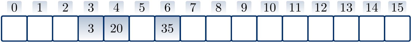
Suppose that $ h’(k) = k $ for integer-valued keys, $ m = 16 $, and we use quadratic probing with the hash function $ h(k) = (h’(k) + \frac{i(i+1)}{2}) \bmod m $ to insert the keys $ 3 $, $ 20 $ and $ 35 $ in a hash table. The result is

If we now remove the key $ 20 $ by simply removing it from the table, the result is

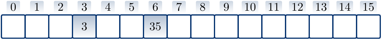
But in this hash table the search operation does not find the key $ 35 $ anymore as it probes the slots $ 3 $ and $ 4 $ only, concluding that the key is not in the set when it sees the free slot at index $ 4 $.

One solution is to replace the remove key with some special “tombstone” key value “del” in the hash table. Search and removal consider these values to be “real keys” but insertion can overwrite them. If the table has too many such tombstones, one should probably “garbage collect” them by rehashing all the values in the same table so that search operations do not perform unnecessary work.

Example

Consider again the hash table of the previous example:

Remove the key $ 20 $ by putting the tombstone value in its place:

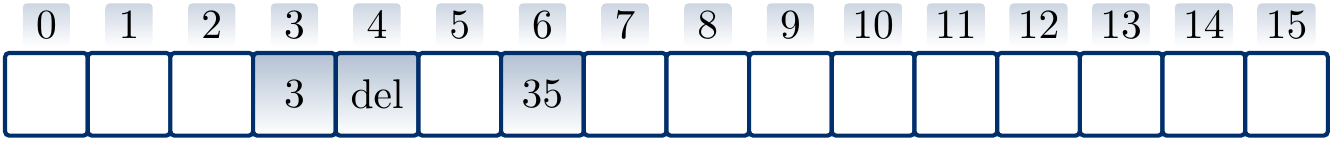
Now the search operation can work unmodified and finds the key $ 35 $ after probing the slots $ 3 $, $ 4 $ and $ 6 $. If we now insert the key $ 19 $, we probe the slots $ 3 $ and $ 4 $ and then insert the key in the slot $ 4 $.

Analysis¶

For the analysis, assume uniform hashing: the probe sequence of each key is equally likely to be any of the $ m! $ permutations of $ \Set{0,1,…,m-1} $. Of the probing methods presented, double hashing is closest to this requirement.

Theorem: 11.6 in Introduction to Algorithms, 3rd ed. (online via Aalto lib)

Under the uniform hashing assumption, the expected number of probings done in the case of an unsuccesfull search is at most $ 1/(1-\alpha) $.

Recall that the load factor $ \alpha $ is less than 1 in a non-full hash-table in open addressing and thus $ 1/(1-\alpha) = 1 + \alpha + \alpha^2 + \alpha^3 + … $. Informal intuitive explanation:

The summand $ 1 $ comes from the fact that at least one probe is done.
The first probed slot was occupied with probability $ \alpha $ and thus a second probe is done with probability $ \alpha $
The first and second probed slot were both occupied with probability $ \alpha^2 $ and thus a third probe is done with probability $ \alpha^2 $
An so on.

Therefore, if we keep the load factor below some constant, then the insertion, search, and removal take constant time on average. For instance, if we keep the load factor at or below $ 0.5 $, then the expected number of probes is at most $ 2 $. Note: the “del” values in the table are accounted to the load factor in this case! If removals are known to occurr often, then separate chaining is probably a better collision resolution approach.

Again, when an open addressing hash-table becomes too full, we perform rehashing: grow the size of the table and reinsert the keys to this new larger table. As in the case of Resizable arrays, the size of the hash table is usually approximately doubled. What is a good value of load factor for triggering rehashing? There is no single best answer but usually one uses something like 0.50 or 0.75 for open addressing.