\(\)
\(%\newcommand{\CLRS}{\href{https://mitpress.mit.edu/books/introduction-algorithms}{Cormen et al}}\)
\(\newcommand{\CLRS}{\href{https://mitpress.mit.edu/books/introduction-algorithms}{Introduction to Algorithms, 3rd ed.} (\href{http://libproxy.aalto.fi/login?url=http://site.ebrary.com/lib/aalto/Doc?id=10397652}{online via Aalto lib})}\)
\(\newcommand{\SW}{\href{http://algs4.cs.princeton.edu/home/}{Algorithms, 4th ed.}}\)
\(%\newcommand{\SW}{\href{http://algs4.cs.princeton.edu/home/}{Sedgewick and Wayne}}\)
\(\)
\(\newcommand{\Java}{\href{http://java.com/en/}{Java}}\)
\(\newcommand{\Python}{\href{https://www.python.org/}{Python}}\)
\(\newcommand{\CPP}{\href{http://www.cplusplus.com/}{C++}}\)
\(\newcommand{\ST}[1]{{\Blue{\textsf{#1}}}}\)
\(\newcommand{\PseudoCode}[1]{{\color{blue}\textsf{#1}}}\)
\(\)
\(%\newcommand{\subheading}[1]{\textbf{\large\color{aaltodgreen}#1}}\)
\(\newcommand{\subheading}[1]{\large{\usebeamercolor[fg]{frametitle} #1}}\)
\(\)
\(\newcommand{\Blue}[1]{{\color{flagblue}#1}}\)
\(\newcommand{\Red}[1]{{\color{aaltored}#1}}\)
\(\newcommand{\Emph}[1]{\emph{\color{flagblue}#1}}\)
\(\)
\(\newcommand{\Engl}[1]{({\em engl.}\ #1)}\)
\(\)
\(\newcommand{\Pointer}{\raisebox{-1ex}{\huge\ding{43}}\ }\)
\(\)
\(\newcommand{\Set}[1]{\{#1\}}\)
\(\newcommand{\Setdef}[2]{\{{#1}\mid{#2}\}}\)
\(\newcommand{\PSet}[1]{\mathcal{P}(#1)}\)
\(\newcommand{\Card}[1]{{\vert{#1}\vert}}\)
\(\newcommand{\Tuple}[1]{(#1)}\)
\(\newcommand{\Implies}{\Rightarrow}\)
\(\newcommand{\Reals}{\mathbb{R}}\)
\(\newcommand{\Seq}[1]{(#1)}\)
\(\newcommand{\Arr}[1]{[#1]}\)
\(\newcommand{\Floor}[1]{{\lfloor{#1}\rfloor}}\)
\(\newcommand{\Ceil}[1]{{\lceil{#1}\rceil}}\)
\(\newcommand{\Path}[1]{(#1)}\)
\(\)
\(%\newcommand{\Lg}{\lg}\)
\(\newcommand{\Lg}{\log_2}\)
\(\)
\(\newcommand{\BigOh}{O}\)
\(%\newcommand{\BigOh}{\mathcal{O}}\)
\(\newcommand{\Oh}[1]{\BigOh(#1)}\)
\(\)
\(\newcommand{\todo}[1]{\Red{\textbf{TO DO: #1}}}\)
\(\)
\(\newcommand{\NULL}{\textsf{null}}\)
\(\)
\(\newcommand{\Insert}{\ensuremath{\textsc{insert}}}\)
\(\newcommand{\Search}{\ensuremath{\textsc{search}}}\)
\(\newcommand{\Delete}{\ensuremath{\textsc{delete}}}\)
\(\newcommand{\Remove}{\ensuremath{\textsc{remove}}}\)
\(\)
\(\newcommand{\Parent}[1]{\mathop{parent}(#1)}\)
\(\)
\(\newcommand{\ALengthOf}[1]{{#1}.\textit{length}}\)
\(\)
\(\newcommand{\TRootOf}[1]{{#1}.\textit{root}}\)
\(\newcommand{\TLChildOf}[1]{{#1}.\textit{leftChild}}\)
\(\newcommand{\TRChildOf}[1]{{#1}.\textit{rightChild}}\)
\(\newcommand{\TNode}{x}\)
\(\newcommand{\TNodeI}{y}\)
\(\newcommand{\TKeyOf}[1]{{#1}.\textit{key}}\)
\(\)
\(\newcommand{\PEnqueue}[2]{{#1}.\textsf{enqueue}(#2)}\)
\(\newcommand{\PDequeue}[1]{{#1}.\textsf{dequeue}()}\)
\(\)
\(\newcommand{\Def}{\mathrel{:=}}\)
\(\)
\(\newcommand{\Eq}{\mathrel{=}}\)
\(\newcommand{\Asgn}{\mathrel{\leftarrow}}\)
\(%\newcommand{\Asgn}{\mathrel{:=}}\)
\(\)
\(%\)
\(% Heaps\)
\(%\)
\(\newcommand{\Downheap}{\textsc{downheap}}\)
\(\newcommand{\Upheap}{\textsc{upheap}}\)
\(\newcommand{\Makeheap}{\textsc{makeheap}}\)
\(\)
\(%\)
\(% Dynamic sets\)
\(%\)
\(\newcommand{\SInsert}[1]{\textsc{insert}(#1)}\)
\(\newcommand{\SSearch}[1]{\textsc{search}(#1)}\)
\(\newcommand{\SDelete}[1]{\textsc{delete}(#1)}\)
\(\newcommand{\SMin}{\textsc{min}()}\)
\(\newcommand{\SMax}{\textsc{max}()}\)
\(\newcommand{\SPredecessor}[1]{\textsc{predecessor}(#1)}\)
\(\newcommand{\SSuccessor}[1]{\textsc{successor}(#1)}\)
\(\)
\(%\)
\(% Union-find\)
\(%\)
\(\newcommand{\UFMS}[1]{\textsc{make-set}(#1)}\)
\(\newcommand{\UFFS}[1]{\textsc{find-set}(#1)}\)
\(\newcommand{\UFCompress}[1]{\textsc{find-and-compress}(#1)}\)
\(\newcommand{\UFUnion}[2]{\textsc{union}(#1,#2)}\)
\(\)
\(\)
\(%\)
\(% Graphs\)
\(%\)
\(\newcommand{\Verts}{V}\)
\(\newcommand{\Vtx}{v}\)
\(\newcommand{\VtxA}{v_1}\)
\(\newcommand{\VtxB}{v_2}\)
\(\newcommand{\VertsA}{V_\textup{A}}\)
\(\newcommand{\VertsB}{V_\textup{B}}\)
\(\newcommand{\Edges}{E}\)
\(\newcommand{\Edge}{e}\)
\(\newcommand{\NofV}{\Card{V}}\)
\(\newcommand{\NofE}{\Card{E}}\)
\(\newcommand{\Graph}{G}\)
\(\)
\(\newcommand{\SCC}{C}\)
\(\newcommand{\GraphSCC}{G^\text{SCC}}\)
\(\newcommand{\VertsSCC}{V^\text{SCC}}\)
\(\newcommand{\EdgesSCC}{E^\text{SCC}}\)
\(\)
\(\newcommand{\GraphT}{G^\text{T}}\)
\(%\newcommand{\VertsT}{V^\textup{T}}\)
\(\newcommand{\EdgesT}{E^\text{T}}\)
\(\)
\(%\)
\(% NP-completeness etc\)
\(%\)
\(\newcommand{\Poly}{\textbf{P}}\)
\(\newcommand{\NP}{\textbf{NP}}\)
\(\newcommand{\PSPACE}{\textbf{PSPACE}}\)
\(\newcommand{\EXPTIME}{\textbf{EXPTIME}}\)
\(\newcommand{\Prob}[1]{\textsf{#1}}\)
\(\newcommand{\SUBSETSUM}{\Prob{subset-sum}}\)
\(\newcommand{\MST}{\Prob{minimum spanning tree}}\)
\(\newcommand{\MSTDEC}{\Prob{minimum spanning tree (decision version)}}\)
\(\newcommand{\ISET}{\Prob{independent set}}\)
\(\newcommand{\SAT}{\Prob{sat}}\)
\(\newcommand{\SATT}{\Prob{3-cnf-sat}}\)
\(\)
\(\newcommand{\VarsOf}[1]{\mathop{vars}(#1)}\)
\(\newcommand{\TA}{\tau}\)
\(\newcommand{\Eval}[2]{\mathop{eval}_{#1}(#2)}\)
\(\newcommand{\Booleans}{\mathbb{B}}\)
\(\)
\(\newcommand{\UWeights}{w}\)
\(\)
\(\newcommand{\False}{\textbf{false}}\)
\(\newcommand{\True}{\textbf{true}}\)
\(\)
\(\newcommand{\SSDP}{\textrm{hasSubset}}\)
\(\)
\(\newcommand{\SUD}[3]{x_{#1,#2,#3}}\)
\(\newcommand{\SUDHints}{H}\)
NP-complete problems
The class \( \NP \) contains both problems that are easy (those in the class \( \Poly \))
as well as
problems for which we do not currently know efficient algorithms (but whose solutions are small and easy to check).
There is a special class of problems in \( \NP \) called
\( \NP \)-complete problems.
They have the property that if any of them can be solved in polynomial time, then all of them can.
In a sense, they are the hardest problems in the class \( \NP \).
And there are lots of such problems.
Definition: Polynomial-time computable reduction
A polynomial-time computable reduction from
a decision problem \( B \) to a decision problem \( A \) is
a function \( R \) from the instances of \( B \) to the instances of \( A \) such that
for each instance \( x \) of \( B \),
\( R(x) \) can be computed in polynomial-time, and
\( x \) is a “yes” instance of \( B \) if and only if \( R(x) \) is a “yes” instance of \( A \).
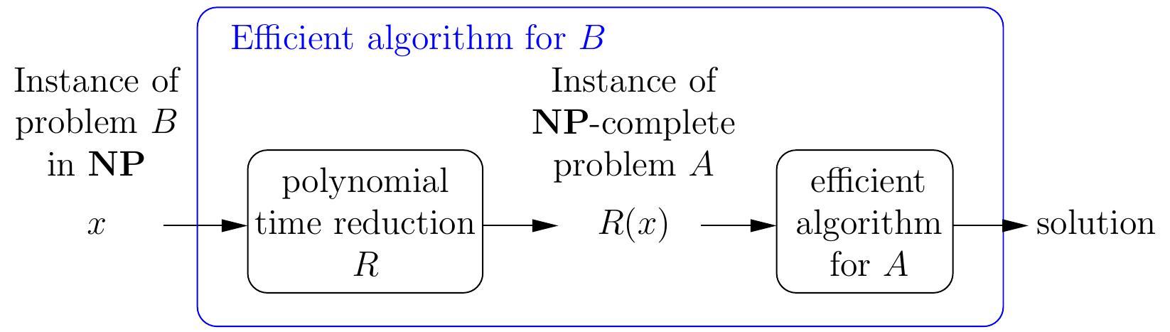
Therefore,
if we have
a polynomial time reduction from \( B \) to \( A \), and
a polynomial-time algorithm solving \( A \),
then we have a polynomial-time algorithm for solving \( B \) as well:
given an instance \( x \) of \( B \), compute \( R(x) \) and
then run the algorithm for \( A \) on \( R(x) \).
Definition: NP-completeness
A problem \( A \) in \( \NP \) is \( \NP \)-complete if
every other problem \( B \) in \( \NP \) can be reduced to it
with a polynomial-time computable reduction.
Therefore,
if an \( \NP \)-complete problem \( A \) can be solved in polynomial time,
then all the problems in \( \NP \) can, and thus
\( \NP \)-complete problems are, in a sense, the most difficult ones in \( \NP \).
We do not know whether \( \NP \)-complete problems can be solved efficiently or not.
The Cook-Levin Theorem
The fact that \( \NP \)-complete problems exist at all was proven by Cook and Levin
in 1970’s.
Theorem: Cook 1971, Levin 1973
\( \SAT{} \) (and \( \SATT{} \)) is \( \NP \)-complete.
Soon after this, Karp [1972] then listed the next 21 \( \NP \)-complete problems.
Since then, hundreds of problems have been shown \( \NP \)-complete.
For instance, \( \Prob{traveling salesperson} \), \( \Prob{generalized Sudokus} \) etc
are all \( \NP \)-complete.
For incomplete lists, one can see
NP-completeness: significance
Of course,
the question of whether \( \Poly = \NP \),
or can \( \NP \)-complete problems be solved in polynomial time,
is a very important open problem in computer science.
In fact, it is one of the seven (of which six are still open)
one million dollar prize Clay Mathematics Institute Millennium Prize problems.
Because there are hundreds of \( \NP \)-complete problems,
the \( \Poly = \NP \) question has practical significance as well.
As Christos Papadimitriou says in his book “Computational complexity”:
There is nothing wrong in trying to prove that an \( \NP \)-complete
problem can be solved in polynomial time.
The point is that without an \( \NP \)-completeness proof one would be trying the same thing without knowing it!
That is, suppose that you have a new problem for which you should develop an algorithm that is always efficient, i.e. runs in polynomial time.
You may end up in trying really hard for very long time,
probably without success,
if the problem turns out to be \( \NP \)-complete or harder.
This is because during the last decades,
lots of very clever people have tried to develop polynomial-time algorithms
for many \( \NP \)-complete problems, but no-one has succeeded so far.