\(\)
\(%\newcommand{\CLRS}{\href{https://mitpress.mit.edu/books/introduction-algorithms}{Cormen et al}}\)
\(\newcommand{\CLRS}{\href{https://mitpress.mit.edu/books/introduction-algorithms}{Introduction to Algorithms, 3rd ed.} (\href{http://libproxy.aalto.fi/login?url=http://site.ebrary.com/lib/aalto/Doc?id=10397652}{online via Aalto lib})}\)
\(\newcommand{\SW}{\href{http://algs4.cs.princeton.edu/home/}{Algorithms, 4th ed.}}\)
\(%\newcommand{\SW}{\href{http://algs4.cs.princeton.edu/home/}{Sedgewick and Wayne}}\)
\(\)
\(\newcommand{\Java}{\href{http://java.com/en/}{Java}}\)
\(\newcommand{\Python}{\href{https://www.python.org/}{Python}}\)
\(\newcommand{\CPP}{\href{http://www.cplusplus.com/}{C++}}\)
\(\newcommand{\ST}[1]{{\Blue{\textsf{#1}}}}\)
\(\newcommand{\PseudoCode}[1]{{\color{blue}\textsf{#1}}}\)
\(\)
\(%\newcommand{\subheading}[1]{\textbf{\large\color{aaltodgreen}#1}}\)
\(\newcommand{\subheading}[1]{\large{\usebeamercolor[fg]{frametitle} #1}}\)
\(\)
\(\newcommand{\Blue}[1]{{\color{flagblue}#1}}\)
\(\newcommand{\Red}[1]{{\color{aaltored}#1}}\)
\(\newcommand{\Emph}[1]{\emph{\color{flagblue}#1}}\)
\(\)
\(\newcommand{\Engl}[1]{({\em engl.}\ #1)}\)
\(\)
\(\newcommand{\Pointer}{\raisebox{-1ex}{\huge\ding{43}}\ }\)
\(\)
\(\newcommand{\Set}[1]{\{#1\}}\)
\(\newcommand{\Setdef}[2]{\{{#1}\mid{#2}\}}\)
\(\newcommand{\PSet}[1]{\mathcal{P}(#1)}\)
\(\newcommand{\Card}[1]{{\vert{#1}\vert}}\)
\(\newcommand{\Tuple}[1]{(#1)}\)
\(\newcommand{\Implies}{\Rightarrow}\)
\(\newcommand{\Reals}{\mathbb{R}}\)
\(\newcommand{\Seq}[1]{(#1)}\)
\(\newcommand{\Arr}[1]{[#1]}\)
\(\newcommand{\Floor}[1]{{\lfloor{#1}\rfloor}}\)
\(\newcommand{\Ceil}[1]{{\lceil{#1}\rceil}}\)
\(\newcommand{\Path}[1]{(#1)}\)
\(\)
\(%\newcommand{\Lg}{\lg}\)
\(\newcommand{\Lg}{\log_2}\)
\(\)
\(\newcommand{\BigOh}{O}\)
\(%\newcommand{\BigOh}{\mathcal{O}}\)
\(\newcommand{\Oh}[1]{\BigOh(#1)}\)
\(\)
\(\newcommand{\todo}[1]{\Red{\textbf{TO DO: #1}}}\)
\(\)
\(\newcommand{\NULL}{\textsf{null}}\)
\(\)
\(\newcommand{\Insert}{\ensuremath{\textsc{insert}}}\)
\(\newcommand{\Search}{\ensuremath{\textsc{search}}}\)
\(\newcommand{\Delete}{\ensuremath{\textsc{delete}}}\)
\(\newcommand{\Remove}{\ensuremath{\textsc{remove}}}\)
\(\)
\(\newcommand{\Parent}[1]{\mathop{parent}(#1)}\)
\(\)
\(\newcommand{\ALengthOf}[1]{{#1}.\textit{length}}\)
\(\)
\(\newcommand{\TRootOf}[1]{{#1}.\textit{root}}\)
\(\newcommand{\TLChildOf}[1]{{#1}.\textit{leftChild}}\)
\(\newcommand{\TRChildOf}[1]{{#1}.\textit{rightChild}}\)
\(\newcommand{\TNode}{x}\)
\(\newcommand{\TNodeI}{y}\)
\(\newcommand{\TKeyOf}[1]{{#1}.\textit{key}}\)
\(\)
\(\newcommand{\PEnqueue}[2]{{#1}.\textsf{enqueue}(#2)}\)
\(\newcommand{\PDequeue}[1]{{#1}.\textsf{dequeue}()}\)
\(\)
\(\newcommand{\Def}{\mathrel{:=}}\)
\(\)
\(\newcommand{\Eq}{\mathrel{=}}\)
\(\newcommand{\Asgn}{\mathrel{\leftarrow}}\)
\(%\newcommand{\Asgn}{\mathrel{:=}}\)
\(\)
\(%\)
\(% Heaps\)
\(%\)
\(\newcommand{\Downheap}{\textsc{downheap}}\)
\(\newcommand{\Upheap}{\textsc{upheap}}\)
\(\newcommand{\Makeheap}{\textsc{makeheap}}\)
\(\)
\(%\)
\(% Dynamic sets\)
\(%\)
\(\newcommand{\SInsert}[1]{\textsc{insert}(#1)}\)
\(\newcommand{\SSearch}[1]{\textsc{search}(#1)}\)
\(\newcommand{\SDelete}[1]{\textsc{delete}(#1)}\)
\(\newcommand{\SMin}{\textsc{min}()}\)
\(\newcommand{\SMax}{\textsc{max}()}\)
\(\newcommand{\SPredecessor}[1]{\textsc{predecessor}(#1)}\)
\(\newcommand{\SSuccessor}[1]{\textsc{successor}(#1)}\)
\(\)
\(%\)
\(% Union-find\)
\(%\)
\(\newcommand{\UFMS}[1]{\textsc{make-set}(#1)}\)
\(\newcommand{\UFFS}[1]{\textsc{find-set}(#1)}\)
\(\newcommand{\UFCompress}[1]{\textsc{find-and-compress}(#1)}\)
\(\newcommand{\UFUnion}[2]{\textsc{union}(#1,#2)}\)
\(\)
\(\)
\(%\)
\(% Graphs\)
\(%\)
\(\newcommand{\Verts}{V}\)
\(\newcommand{\Vtx}{v}\)
\(\newcommand{\VtxA}{v_1}\)
\(\newcommand{\VtxB}{v_2}\)
\(\newcommand{\VertsA}{V_\textup{A}}\)
\(\newcommand{\VertsB}{V_\textup{B}}\)
\(\newcommand{\Edges}{E}\)
\(\newcommand{\Edge}{e}\)
\(\newcommand{\NofV}{\Card{V}}\)
\(\newcommand{\NofE}{\Card{E}}\)
\(\newcommand{\Graph}{G}\)
\(\)
\(\newcommand{\SCC}{C}\)
\(\newcommand{\GraphSCC}{G^\text{SCC}}\)
\(\newcommand{\VertsSCC}{V^\text{SCC}}\)
\(\newcommand{\EdgesSCC}{E^\text{SCC}}\)
\(\)
\(\newcommand{\GraphT}{G^\text{T}}\)
\(%\newcommand{\VertsT}{V^\textup{T}}\)
\(\newcommand{\EdgesT}{E^\text{T}}\)
\(\)
\(%\)
\(% NP-completeness etc\)
\(%\)
\(\newcommand{\Poly}{\textbf{P}}\)
\(\newcommand{\NP}{\textbf{NP}}\)
\(\newcommand{\PSPACE}{\textbf{PSPACE}}\)
\(\newcommand{\EXPTIME}{\textbf{EXPTIME}}\)
\(\newcommand{\Prob}[1]{\textsf{#1}}\)
\(\newcommand{\SUBSETSUM}{\Prob{subset-sum}}\)
\(\newcommand{\MST}{\Prob{minimum spanning tree}}\)
\(\newcommand{\MSTDEC}{\Prob{minimum spanning tree (decision version)}}\)
\(\newcommand{\ISET}{\Prob{independent set}}\)
\(\newcommand{\SAT}{\Prob{sat}}\)
\(\newcommand{\SATT}{\Prob{3-cnf-sat}}\)
\(\)
\(\newcommand{\VarsOf}[1]{\mathop{vars}(#1)}\)
\(\newcommand{\TA}{\tau}\)
\(\newcommand{\Eval}[2]{\mathop{eval}_{#1}(#2)}\)
\(\newcommand{\Booleans}{\mathbb{B}}\)
\(\)
\(\newcommand{\UWeights}{w}\)
\(\)
\(\newcommand{\False}{\textbf{false}}\)
\(\newcommand{\True}{\textbf{true}}\)
\(\)
\(\newcommand{\SSDP}{\textrm{hasSubset}}\)
\(\)
\(\newcommand{\SUD}[3]{x_{#1,#2,#3}}\)
\(\newcommand{\SUDHints}{H}\)
Computational problems
A computational problem consists of a description of
what the possible inputs, called instances of the problem, are
and
what is the question that should be answered on such inputs.
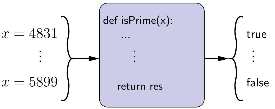
As an example, the problem of testing whether an integer is a prime number
can be expressed as the following computational problem.
Definition: \( \Prob{Primality} \) problem
Instance: A positive integer \( x \).
Question: Is \( x \) a prime number?
To solve this problem, one has to develop an algorithm
that gives the correct answer for all possible input instances.
A problem is decidable (or “computable”, or sometimes “recursive” due to historical reasons)
if there is an algorithm that can, for all possible instances,
answer the question.
For instance, the \( \Prob{Primality} \) problem is decidable;
a simple but inefficient way to test whether \( x \) is a prime number is
to check, for all integers \( i \in [2..\lfloor\sqrt{x}\rfloor] \),
that \( i \) does not divide \( x \).
In a decision problem the answer is either “no” or “yes”.
Definition: The \( \SUBSETSUM \) problem
Instance: A set \( S \) of integers and a target value \( t \).
Question: Does \( S \) have a subset \( S’ \subseteq S \) such that \( \sum_{s \in S’}s = t \)?
In a function problem the answer is either
Definition: The \( \SUBSETSUM \) problem (function version)
Instance: A set \( S \) of integers and a target value \( t \).
Question: Give a subset \( S’ \subseteq S \) such that \( \sum_{s \in S’}s = t \) if such exists.
Mathematically, a computational problem with a no/yes answer
can be defined as the set of input strings for which the answer is “yes”.
Problems with a more complex answers can be defined as (partial) functions.
These formal aspects will be studied more in the Aalto course
“CS-C2160 Theory of Computation”.
In optimization problems one has to find an/the optimal solution.
Definition: \( \MST \) problem
Instance: A connected edge-weighted and undirected graph \( G \).
Question: Give a minimum spanning tree of the graph.
For an optimization problem there usually is a corresponding
decision problem with some threshold value for the solution
(is there an “at least this good solution”?).
Definition: \( \MSTDEC \) problem
Instance: A connected edge-weighted and undirected graph \( G \) and an integer \( k \).
Question: Does the graph have a spanning tree of weight \( k \) or less?
The full optimization problem is at least as hard as this decision
version because an optimal solution gives immediately
the solution for the decision version as well.
In computational complexity theory,
the set of decidable problems can be divided in many smaller complexity classes:
\( \Poly \) — problems that can be solved in polynomial time (\( \approx \) always efficiently) with algorithms
\( \NP \) — problems whose solution can be verified in polynomial time
(or that can solved with non-deterministic machines in polynomial time)
\( \PSPACE \) — problems that can be solved with a polynomial amount of extra space (possibly in exponential time)
\( \EXPTIME \) — problems that can be solved in exponential time in memory
and many more…
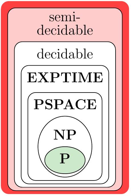
In this round and course, we focus on problems in the classes \( \Poly \) and \( \NP \).
More difficult problems are encountered, for instance, in the “Artificial Intelligence” course.