Dynamic programming¶

Dynamic programming is a generic algorithm design technique. It is applicable for solving many optimization problems, where we want to find the best solution for some problem. In a nutshell, dynamic programming could be described as “exhaustive recursive search with sub-problem solution reuse”. The term “dynamic programming” itself is due to historical reasons, see the text in this Wikipedia page.

The generic idea in dynamic programming is as follows.

Define the (optimal) solutions for the problem by using (optimal) solutions for some sub-problems of the original problem. This leads to a recursive definition for the (optimal) solutions.
Check if the sub-problems occur many times in the expansion of the recursive definition.
If they do, apply memoization when evaluating the recursive definition. That is, instead of recomputing the same sub-problems again and again, store their solutions in a map/table/etc and reuse the solutions whenever possible.

(If they don’t, the sub-problems don’t “overlap” and dynamic programming is not applicable. Sometimes it is possible to make an alternative recursive definition that has overlapping sub-problems.)

Let us now practise this proceduce by considering three increasingly complex problems and showing how they can be solved with dynamic programming.

Example I: Fibonacci numbers¶

Let’s start with a very simple example from previous courses. The Fibonacci numbers sequence $ F_n = 0,1,1,2,3,5,8,… $ is defined recursively by $$F_0 = 0, F_1 = 1, \text{ and } F_n = F_{n-1}+F_{n-2} \text{ for } n \ge 2$$ It is rather easy to implement a program that computes the $ n $th Fibonacci number by using recursion:

def fib(n: Int): BigInt = {
  require(n >= 0)
  if(n == 0) 0
  else if(n == 1) 1
  else fib(n-1) + fib(n-2)
}

The figure below shows the call tree, also called recursion tree, when computing fib(6):

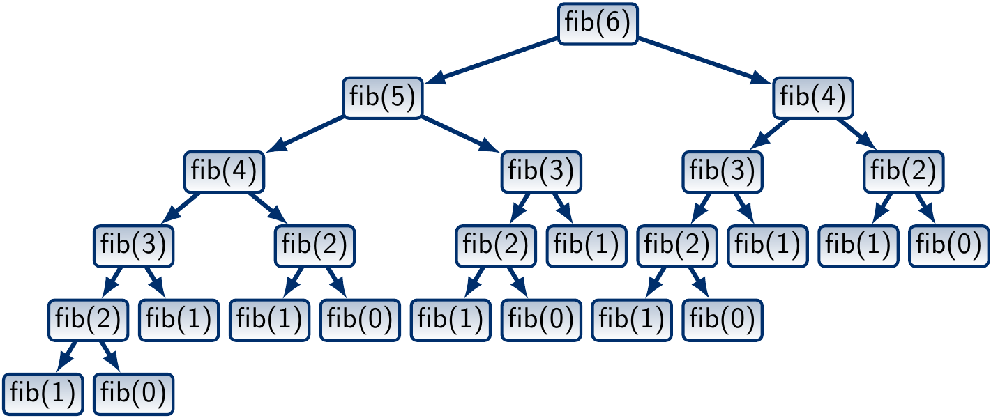
Observe that many (pure) function invocations occur multiple times. For instance, the call fib(3) occurs three times. In other words, the same sub-problem fib(i) can be solved many times. This is reflected in the running time: computing the 45th Fibonacci number 1134903170 takes almost 50 seconds on a rather standard desktop machine:

scala> measureCpuTime {fib(45) }
res2: (BigInt, Double) = (1134903170,49.203652944)

What is the asymptotic running time of this algorithm? Assuming that addition of numbers could be done in constant time, we get the following recurrence: $$T(n) = T(n-2)+T(n-1)+\Theta(1)$$ As $ T(n) $ is non-decreasing, $ T(n) \ge 2 T(n-2) + \Theta(1) $ and thus $ T(n) = \Omega(2^{n/2}) $. Therefore, the algorithm takes at least exponential time.

The above analysis is actually not very precise because the addition is not done in constant time. This is because $$F_n = \frac{\varphi^n-(-\frac{1}{\varphi})^n}{\sqrt{5}} = \frac{\varphi^n}{\sqrt{5}}-\frac{(-\frac{1}{\varphi})^n}{\sqrt{5}} = \Omega(\varphi^n)$$ where $ \varphi= 1.6180339887… $ is the golden ratio. This means that the binary representations of the numbers in $ F_n $ grow linearly in $ n $. Therefore, the $ \Theta(1) $ term in the recurrence should be $ \Theta(n) $.

Applying dynamic programming¶

Instead of recomputing the values fib(i) over and over again, we can memoize the values in a map and reuse them whenever possible. In Scala, a basic version of memoization is easy to obtain by just using a mutable map that maps the sub-problems to their solutions. In this case, the map associates the argument i to the value fib(i).

def fibonacci(n: Int): BigInt = {
  require(n >= 0)
  val m = collection.mutable.Map[Int, BigInt]()     // ADDED
  def fib(i: Int): BigInt = m.getOrElseUpdate(i, {  // CHANGED
    if(i == 0) 0
    else if(i == 1) 1
    else fib(i-1) + fib(i-2)
  })
  fib(n)
}

The running time is dramatically improved, and we can compute much larger Fibonacci numbers much faster:

scala> measureCpuTime { fibonacci(1000) }
res14: (BigInt, Double) = (<A number with 209 digits>,0.001016623)

This memoization, or sub-solution caching, is a key component in dynamic programming. Let’s study the call tree for fib(6) with memoization:

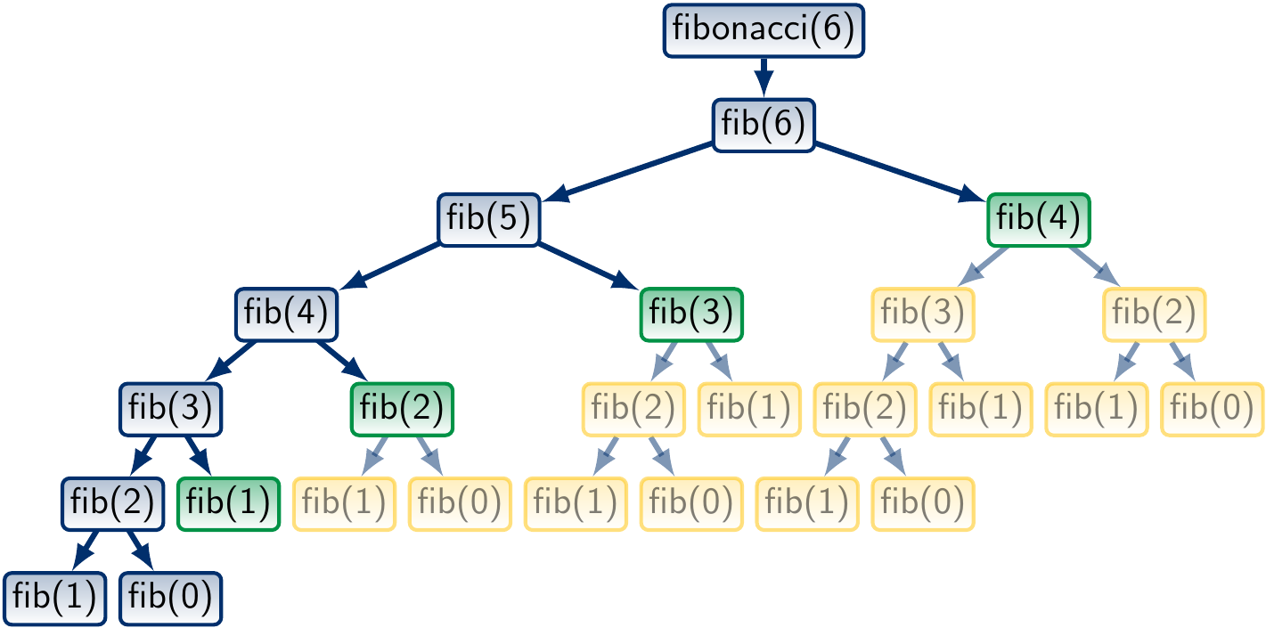
Here the green nodes are those whose value is found in the memoization map, and whose subtrees, marked in yellow, are not traversed at all. We observe that a significant part of the call tree is not traversed at all.

What then is the running time of this improved algorithm? It is the number of different function invocations times the amount of the time spent in each. Assuming constant-time addition and map lookup+update (as we have seen earlier in this course, map lookup+update is actually $ \Oh{\log n} $ or $ \Oh{1} $ on average when tree maps or hash maps are used), the running time is $$n \times \Theta(1) = \Theta(n)$$ No recurrences were need in computing this. If we want to be more precise and take into account the linear time of adding two $ \Theta(n) $ bit numbers, then the worst-case running time is $$T(n) = T(n-1)+\Theta(n)=\Theta(n^2)$$ The memory consumption of the algorithm $ \Theta(n^2) $ as well because the map stores $ n $ numbers with $ \Oh{n} $ bits each.

However, even with memoization, the recursive version is not tail recursive and can thus exhaust stack frame memory (recall the CS-A1120 Programming 2 course). To fix this problem, we can skip the recursion phase and simply perform the same computations iteratively bottom-up.

That is, we store the fib(i) values in an array.

We start by setting set fib(0) = 0 and fib(1) = 1.
Next, we compute fib(2) from fib(1) and fib(0).
Next, we compute fib(3) from fib(2) and fib(1).
And so on

Here is an implementation in Scala:

def fibonacci(n: Int): BigInt = {
  require(n >= 0)
  val fib = new Array[BigInt](n+1 max 2)
  fib(0) = 0
  fib(1) = 1
  for(i <- 2 to n)
    fib(i) = fib(i-2) + fib(i-1)
  fib(n)
}

scala> measureCpuTime { fibonacci(1000) }
res17: (BigInt, Double) = (<A number with 209 digits>,7.05329E-4)

Now the lookup+update in arrays is guaranteed to work in constant time. However, the memory consumption is still $ \Theta(n^2) $.

In this simple example of Fibonacci numbers, we actually only have to remember the last two values and can thus reduce the amount of memory needed. Starting from $ F_0 $ and $ F_1 $, we simply iterate to $ F_n $:

def fibonacci(n: Int): BigInt = {
  require(n >= 0)
  if(n == 0) return 0
  var fibPrev = BigInt(0)
  var fib = BigInt(1)
  for(i <- 1 until n) {
    val fibNew = fibPrev + fib
    fibPrev = fib
    fib = fibNew
  }
  fib
}

scala> measureCpuTime { fib(1000) }
res48: (BigInt, Double) = (<A number with 209 digits>,6.0929E-4)

Now the memory consumption is reduced to $ \Theta(n) $.

The same can also be written in the functional style as follows:

def fibonacci(n: Int): BigInt = {
  require(n >= 0)
  if(n == 0)
    0
  else
    (1 until n)
    .foldLeft(BigInt(0),BigInt(1))(
      {case ((fibPrev,fib), _) => (fib, fibPrev+fib)}
    )._2
}

Recap: typical steps in solving problems with dynamic programming¶

After the first example, we can now recap the main steps in applying dynamic programming to solving a computational problem.

Define the (optimal) solutions based on the (optimal) solutions to sub-problems. This leads to a recursive definition for the (optimal) solutions.

In the Fibonacci example, there was no optimality requirement, and the recursive definition was already given.
Check if the sub-solutions occur many times in the call trees.
If they do, apply memoization in the recursive version or build an iterative version using arrays to store sub-solutions.

In the Fibonacci example this was the case and we obtained substantial improvements in performance when compared to the plain recursive version.

Example II: Rod cutting¶

Let’s consider a second example where the recursive definition is not given but we’ve to figure out one. Study the following optimization problem:

Problem: The rod cutting problem

We are given a rod of length $ n $ and an array $ \Seq{\Price{1},…,\Price{n}} $ of prices, each $ \Price{i} $ telling the amount of money we get if we sell a rod piece of length $ i $. We can cut the rod in pieces and making cuts is free.

What is the best way to cut the rod so that we get the maximum profit?

Example

Suppose that we have a rod of length $ 4 $ and that the prices are

$ 2 $ credits for rod units of length $ 1 $,
$ 4 $ credits for rod units of length $ 2 $,
$ 7 $ credits for rod units of length $ 3 $, and
$ 8 $ credits for rod units of length $ 4 $.

The best way to cut our rod is to make one piece of length $ 1 $ and one of length $ 3 $. Selling them gives us $ 9 $ credits.

Recursive formulation¶

How do we define the optimal solutions recursively? That is, how to cut a rod of length $ n $ to get maximum profit? Denote the maximum profit by $ \Profit{n} $. Now it is quite easy to observe that $ \Profit{n} $ is the maximum of the following profits:

Cut away a piece of length $ 1 $ and then cut the remaining rod of length $ n-1 $ in the best way $ \Rightarrow $ the profit is $ \Price{1} + \Profit{n-1} $.
Cut away a piece of length $ 2 $ and then cut the remaining rod of length $ n-2 $ in the best way $ \Rightarrow $ the profit is $ \Price{2} + \Profit{n-2} $.
and so on
Cut away a piece of length $ n-1 $ and then cut the remaining rod of length $ 1 $ in the best way $ \Rightarrow $ the profit is $ \Price{n-1} + \Profit{1} $.
Make no cuts, the profit is $ \Price{n} $.

Therefore, we can formulate $ \Profit{n} $ as $$\Profit{n} = \max_{i = 1,…,n} (\Price{i} + \Profit{n-i})$$ with the base case $ \Profit{0} = 0 $ so that the last “no cuts” case is treated uniformly. Again, once we have the recursive formulation, implementation is straightforward. For istance, in Scala we can write the following recursive function:

def bestCut(n: Int, prices: Array[Int]) = {
  require(prices.length >= n+1)
  require(prices(0) == 0 && prices.forall(_ >= 0))
  def cut(k: Int): Long = {
    if(k == 0) 0
    else {
      var best: Long = -1
      for(i <- 1 to k)
	best = best max (prices(i) + cut(k - i))
      best
    }
  }
  cut(n)
}

The same in functional style:

def bestCut(n: Int, prices: Array[Int]) = {
  require(prices.length >= n+1)
  require(prices(0) == 0 && prices.forall(_ >= 0))
  def cut(k: Int): Long = {
    if(k == 0) 0
    else (1 to k).iterator.map(i => prices(i) + cut(k - i)).max
  }
  cut(n)
}

Question: why is iterator used in the code above?

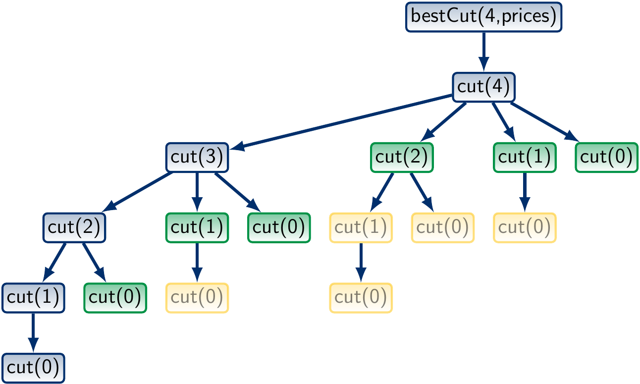
The call tree when $ n = 4 $ looks like this:

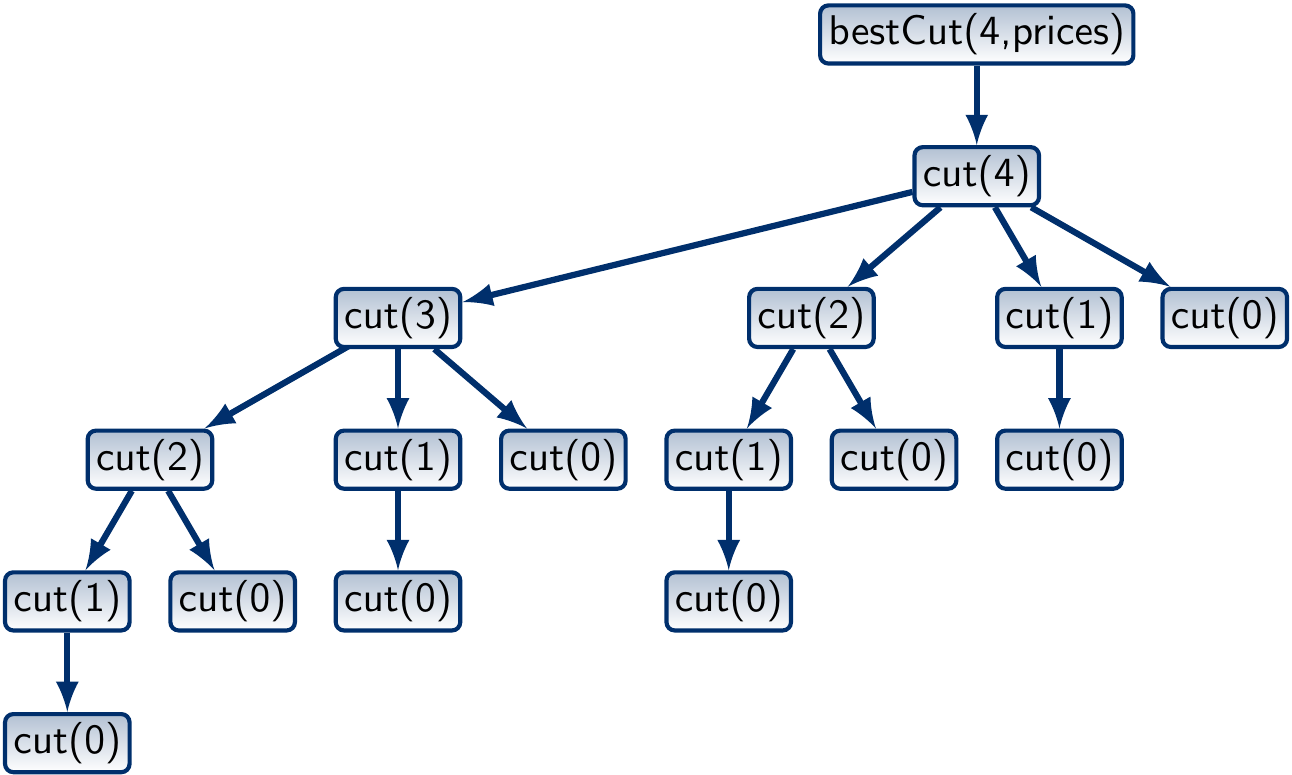
What is the worst-case running time of the program? In a rod of length $ n $, there are $ n-1 $ places where we can make a cut. Therefore, there are $ 2^{n-1} $ ways to cut the rod. As the algorithm generates each of them, its worst-case running time is $ \Theta(2^n) $.

We could have “optimized” the program by always taking the cuts of length 1 first, then those of length 2 and so on in our recursive definition. In this case, the number of ways the rod can be cut is the same as the number of ways a natural number $ n $ can be partitioned and is called the partition function $ p(n) $. Again, $ p(n) $ grows faster than any polynomial in $ n $ and the resulting algorithm would not be very efficient.

Dynamic programming with memoization¶

As in our previous example of Fibonacci numbers, we can use memoization to avoid solving the same sub-problems multiple times:

def bestCut(n: Int, prices: Array[Int]) = {
  require(prices.length >= n+1)
  require(prices(0) == 0 && prices.forall(_ >= 0))
  val m = collection.mutable.Map[Int, Long]() // ADDED
  def cut(k: Int): Long = m.getOrElseUpdate(k, {  // CHANGED
    if(k == 0) 0
    else {
      var best: Long = -1
      for(i <- 1 to k)
	best = best max (prices(i) + cut(k - i))
      best
    }
  })
  cut(n)
}

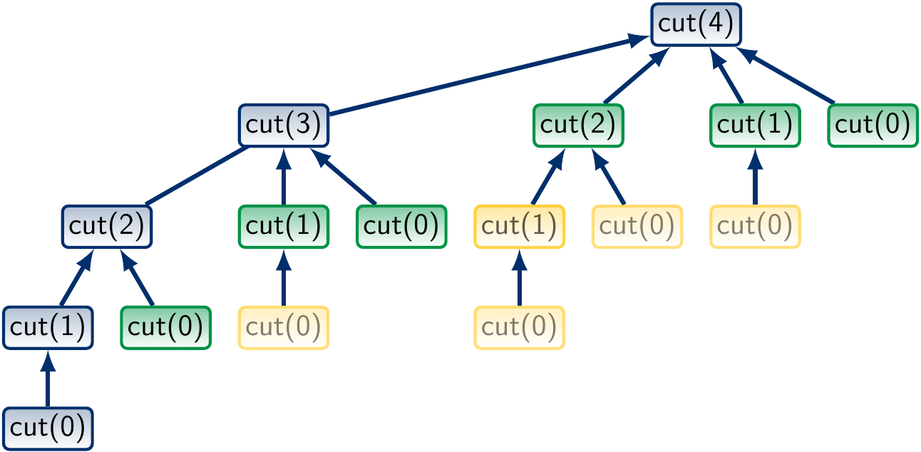
Now the call tree for $ n = 4 $ is

where the green function calls are found in the memoization map and yellow ones are never invoked. The worst-case running time is obtained with the recurrences $ T(0) = \Theta(1) $ and $ T(n) = \Theta(n) + T(n-1) $. Therefore, $ T(n) = \Theta(n^2) $. The term $ \Theta(n) $ above is due to the for-loop over $ n $ values for finding the maximum one.

Constructing the solution¶

In the rod cutting problem, we are not only interested in the optimal price value but the also in how it can be obtained, i.e., how the rod should be cut in order to get the maximum profit. To have this information, we can simply record, in each call inner(k), not only the best profit but also which cutting produced that. There could be many cuttings that produce the best profit but we record only one because the number of such cuttings can be very large. The idea as code

def bestCut(n: Int, prices: Array[Int]) = {
  require(prices.length >= n+1)
  require(prices(0) == 0 && prices.forall(_ >= 0))
  val m = mutable.Map[Int, (Long, List[Int])]() // CHANGED
  def cut(k: Int): (Long, List[Int]) = m.getOrElseUpdate(k, {
    if(k == 0) (0, Nil)
    else {
      var best: Long = -1
      var bestCuts: List[Int] = null       // ADDED
      for(i <- 1 to k) {
	val (subValue, subCuts) = cut(k - i)
	if(subValue + prices(i) > best) {
	  best = subValue + prices(i)
	  bestCuts = i :: subCuts          // ADDED
	}
      }
      (best, bestCuts)  // CHANGED
    }
  })
  cut(n)
}

Observe that we used linked lists for storing the cut sequences. In this way, the map entry for each inner(k) stores only a constant amount of data: the currently added piece length and a reference to the sub-problem solution. The running time of the algorithm remains to be $ \Oh{n^2} $.

An iterative bottom-up version¶

As in the Fibonacci numbers example, we can perform the same iteratively bottom-up. Again, we compute and store the results of the cut(i) calls in an array.

First, we set cut(0) = 0.
Next, compute cut(1) from cut(0).
Next, compute cut(2) from cut(0) and cut(1).
Next, compute cut(3) from cut(0), cut(1) and cut(2).
And so on.

An implementation in Scala:

def bestCut(n: Int, prices: Array[Int]) = {
  require(prices.length >= n+1)
  require(prices(0) == 0 && prices.forall(_ >= 0))
  val cut = new Array[(Long, List[Int])](n+1)
  cut(0) = (0, Nil) // The base case
  for(k <- 1 to n) {
    var best: Long = -1
    var bestCuts: List[Int] = null
    for(i <- 1 to k) {
      val (subValue, subCuts) = cut(k - i)
      if(subValue + prices(i) > best) {
	best = subValue + prices(i)
	bestCuts = i :: subCuts
      }
    }
    cut(k) = (best, bestCuts)
  }
  cut(n)
}

As in the memoization version, the memory consumption is $ \Theta(n) $.

To recap: when is dynamic programming applicable? In general, dynamic programming can be applied when

we can defined the (optimal) solutions by using smaller (optimal) sub-problem solutions, and
the sub-problems overlap, meaning that the same sub-problem can be used multiple times.

Example III: Longest common subsequence¶

Let’s repeat the same process one more time. Now consider two sequences of symbols, say $ \LCSA = \Seq{\LCSa1,…,\LCSa{n}} $ and $ \LCSB = \Seq{\LCSb1,…,\LCSb{m}} $. They could be DNA sequences, written texts etc. We are interested in finding out how “similar” the sequences are. Naturally, there are many possible measures for “similarity”, but here we consider the following definitions:

A common subsequence of $ \LCSA $ and $ \LCSB $ is a sequence $ \LCSO = \Seq{\LCSo{1},…,\LCSo{k}} $ whose elements appear in the same order in both $ \LCSA $ and in $ \LCSB $.
A longest common subsequence (LCS) is a common subsequence of maximal length.

The longer the longest common subsequence(s) are, the more similar the strings are considered to be. The longest common subsequence problem is thus:

Given two sequences, find one of their longest common subsequences.

Example

Consider the sequences $ \LCSA = \Seq{A,C,G,T,A,T} $ and $ \LCSB = \Seq{A,T,G,T,C,T} $. Their (unique) longest common subsequence is $ \Seq{A,G,T,T} $.

Note

Note the longest common subsequences are not necessarily unique. For instance, take the sequences $ \LCSA = \Seq{C,C,C,T,T,T} $ and $ \LCSB = \Seq{T,T,T,C,C,C} $. Their LCSs are $ \Seq{C,C,C} $ and $ \Seq{T,T,T} $

A simple approach to solve the length of an LCS of sequences (and to find one) would be to

generate, in a longest-first order, all the subsequences of one sequence, and
check, for each, whether it is also a subsequence of the other.

Of course, this would be very inefficient as there are exponentially many subsequences.

Recursive definition¶

Again, in order to use dynamic programming, we have to develop a recursive definition for building optimal solutions from optimal solutions to sub-problems. Given the sequences $ \LCSA = \Seq{\LCSa1,…,\LCSa{n}} $ and $ \LCSB = \Seq{\LCSb1,…,\LCSb{m}} $, we use the definitions

$ \LCSAP{i} = \Seq{\LCSa1,…,\LCSa{i}} $ for $ 0 \le i \le n $ and
$ \LCSBP{j} = \Seq{\LCSb1,…,\LCSb{j}} $ for $ 0 \le j \le m $

to the denote prefixes of $ \LCSA $ and $ \LCSB $. Observe that $ \LCSA = \LCSAP{n} $ and $ \LCSB = \LCSBP{m} $.

We obtain a recursive definition for the LCS problem by studying the last symbols in the prefix sequences $ \LCSAP{i} = \Seq{\LCSa1,…,\LCSa{i}} $ and $ \LCSBP{j} = \Seq{\LCSb1,…,\LCSb{j}} $:

If $ \LCSa{i} = \LCSb{j} $, then we obtain an LCS of $ \LCSAP{i} $ and $ \LCSBP{j} $ by taking an LCS of $ \LCSAP{i-1} $ and $ \LCSBP{j-1} $ and concatenating it with $ \LCSa{i} $.
If $ \LCSa{i} \neq \LCSb{j} $ and $ \LCSO $ is an LCS of $ \LCSAP{i} $ and $ \LCSBP{j} $, then
- if $ \LCSa{i} $ is not the last symbol of $ \LCSO $, then $ \LCSO $ is an LCS of $ \LCSAP{i-1} $ and $ \LCSBP{j} $, and
- if $ \LCSb{j} $ is not the last symbol of $ \LCSO $, then $ \LCSO $ is an LCS of $ \LCSAP{i} $ and $ \LCSBP{j-1} $.

Naturally, when $ i = 0 $ or $ j = 0 $, the LCS is the empty sequence with length $ 0 $. These form the base cases for the recursive definition.

Example

Let’s illustrate the cases in the definition.

If $ \LCSAP{6} = \Seq{A,C,G,T,A,T} $ and $ \LCSBP{5} = \Seq{A,G,C,C,T} $, then their LCSs are $ \Seq{A,C,T} $ and $ \Seq{A, G, T} $. Both are obtained from the two LCSs $ \Seq{A,C} $ and $ \Seq{A,G} $ of $ \LCSAP{5}=\Seq{A,C,G,T,A} $ and $ \LCSBP{4}=\Seq{A,G,C,C} $ by concatenating them with the last symbol $ T $.
If $ \LCSAP{6} = \Seq{A,G,C,A,T,C} $ and $ \LCSBP{7} = \Seq{A,C,G,T,A,T,G} $, then their LCSs are $ \Seq{A,C,A,T} $ and $ \Seq{A,G,A,T} $. Neither contain $ C $ as the last symbol and both are an LCS of $ \LCSAP{5} = \Seq{A,G,C,A,T} $ and $ \LCSBP{7} = \Seq{A,C,G,T,A,T} $.
If $ \LCSAP{5} = \Seq{A,G,C,A,C} $ and $ \LCSBP{6} = \Seq{A,C,G,T,A,T} $, then their LCSs are $ \Seq{A,C,A} $ and $ \Seq{A,G,A} $. Neither contain $ T $ as the last symbol and both are an LCS of $ \LCSAP{5} = \Seq{A,G,C,A,C} $ and $ \LCSBP{5} = \Seq{A,C,G,T,A} $.

Again, once we have a recursive definition, an implementation follows without too much effort:

def getLCS(x: String, y: String) = {
  def lcs(i: Int, j: Int): String = {
    if(i == 0 || j == 0) ""
    else if(x(i-1) == y(j-1)) // Observe indexing of x and y!
      lcs(i-1, j-1) + x(i-1)
    else {
      val dropX = lcs(i-1, j)
      val dropY = lcs(i, j-1)
      if(dropX.length >= dropY.length) dropX else dropY
    }
  }
  lcs(x.length, y.length)
}

Observe that string indexing starts from 0 in Scala, not from 1 as in the mathematical definitions above. Again, this simple implementation implementation has exponential running time in the worst case.

scala> timer.measureCpuTime {getLCS("eaaaaaaaaaabbbbbb", "eccccccccccdddddd") }
res1: (String, Double) = (e,37.03632908)

But for some inputs, such as getLCS(“abcab”,”cab”), it is quite fast; why is this the case?

Note also that concatenating a single character at the end of a string is not a constant-time operation; thus the naive version above is not a very optimal solution in this sense either.

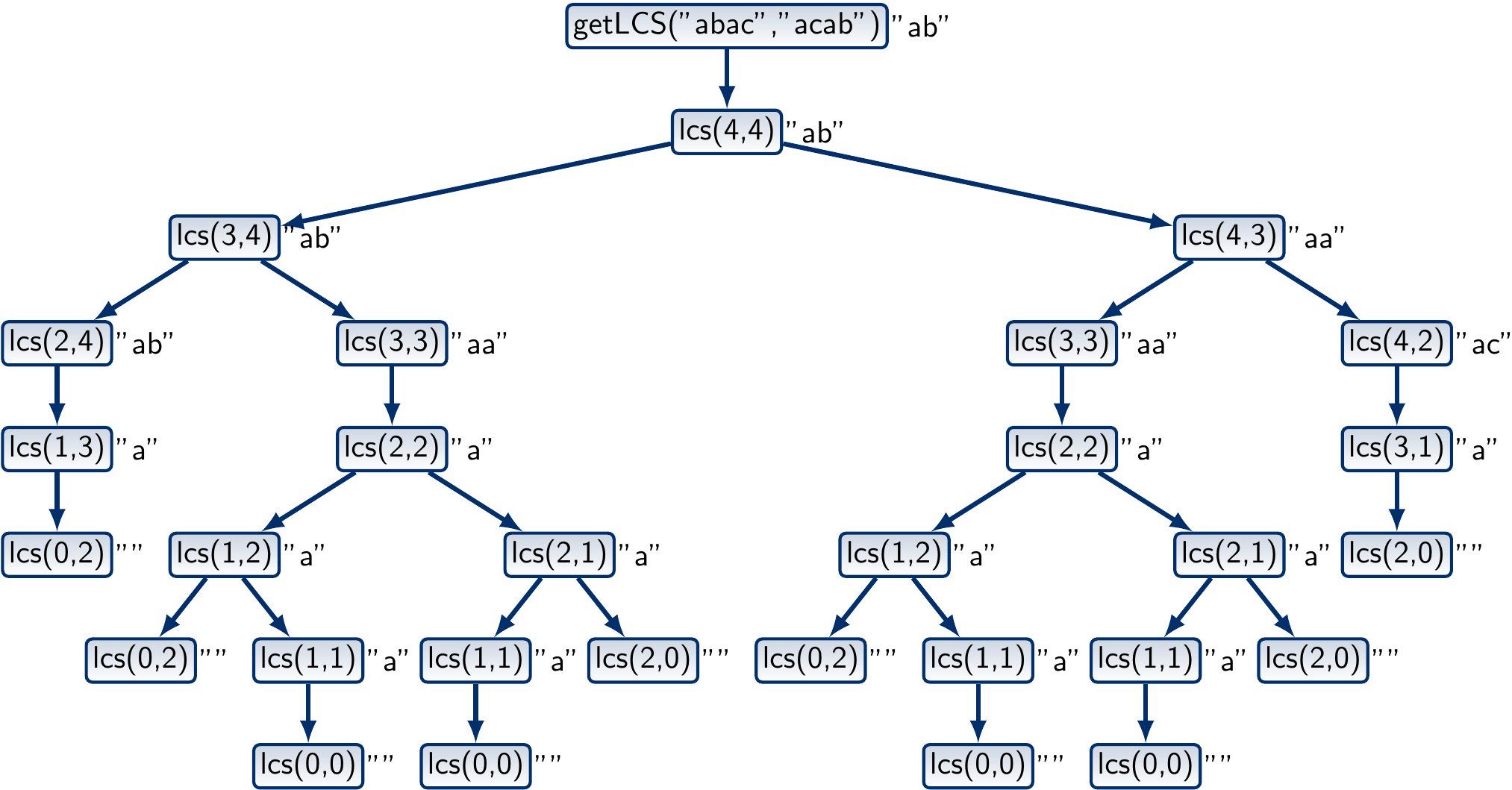
The call tree for the sequences “abac” and “acab” is shown below. To improve readability, the return values of the function calls are also shown on the right of the nodes.

Dynamic programming with memoization¶

Again, we can apply memoization:

def getLCS(x: String, y: String) = {
  val mem = collection.mutable.HashMap[(Int,Int), String]() // ADDED
  def lcs(i: Int, j: Int): String = mem.getOrElseUpdate((i,j), { // CHANGED
    if(i == 0 || j == 0) ""
    else if(x(i-1) == y(j-1))
      lcs(i-1, j-1) + x(i-1)
    else {
      val dropX = lcs(i-1, j)
      val dropY = lcs(i, j-1)
      if(dropX.length >= dropY.length) dropX else dropY
    }
  })
  lcs(x.length, y.length)
}

This version has much better running time:

scala> timer.measureCpuTime {getLCS("eaaaaaaaaaabbbbbb", "eccccccccccdddddd") }
res1: (String, Double) = (e,0.001717177)

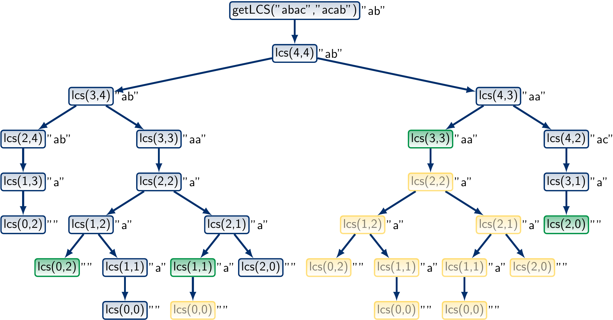
The call tree for the sequences “abac” and “acab” now looks like this:

What is the worst-case running time and memory consumption of the memoization approach? Let $ n $ be the length of the string $ x $ and $ m $ be the length of $ y $. There are $ nm $ possible inner function calls of the form lcs(i,j). Due to the non-constant-time string append operation, each can take time $ \Oh{l} $, where $ l $ is the length of LCSs of $ x $ and $ y $. Thus the worst-case running time is $ \Oh{n m l} $.

Similarly, the worst-case memory consumption $ \Oh{n m l} $ as at most $ nm $ strings are stored in the mem map, and they are of length $ \Oh{l} $.

We can improve running time and memory consumption to $ \Oh{n m} $ as follows.

First, we compute sub-solution lengths only in the mem map.
Then, based on the sub-solution lengths, construct one solution.

This is based on the following observation. Suppose that we are on the call lcs(i,j), initally $ i=n $ and $ j=m $.

If $ x_i = y_j $, then we know that the solution has the symbol $ x_i $ as the last one, and that the first ones are found by calling lcs(i-1,j-1).
Otherwise, mem(i,j) is the maximum of mem(i-1,j) and mem(i,j-1). If mem(i,j) is equal to mem(i-1,j), then an LCS of $ \LCSAP{i} $ and $ \LCSBP{j} $ is found by calling lcs(i-1,j).

And if mem(i,j) is equal to mem(i,j-1), then an LCS of $ \LCSAP{i} $ and $ \LCSBP{j} $ is found by calling lcs(i,j-1). A Scala implementation of this idea is shown here:

def getLCS(x: String, y: String) = {
  // Compute sub-solution lengths in mem
  val mem = collection.mutable.HashMap[(Int,Int), Int]()
  def lcs(i: Int, j: Int): Int = mem.getOrElseUpdate((i,j), {
    if(i == 0 || j == 0) 0
    else if(x(i-1) == y(j-1)) lcs(i-1, j-1) + 1
    else lcs(i-1, j) max lcs(i, j-1)
  })
  lcs(x.length, y.length)
  // Construct one concrete LCS
  def construct(i: Int, j: Int): List[Char] = {
    if(i == 0 || j == 0) Nil
    else if(x(i-1) == y(j-1)) x(i-1) :: construct(i-1,j-1)
    else if(mem(i,j) == mem(i-1,j)) construct(i-1,j)
    else construct(i,j-1)
  }
  construct(x.length, y.length).reverse.mkString("")
}

Now each lcs(i,j) call takes constant time, and ony a constant amount of data is stored in each mem(i,j) entry. Furthermore, the solution construction phase works in time and space $ \Oh{\max\{n,m\}} $. Thus the worst-case running time and memory consumption are $ \Oh{n m} $.

An iterative bottom-up version¶

As stated earlier, the main problem with recursive implementations, even when memoization is used, is that the recursion depth can be large and cause stack overflow errors in systems (such as Java VM) with a fixed amount of memory allocated for the call stack. For instance, if we apply the recursive Scala program above on two strings with thousands of characters having a long LCS, a stack overflow error will occur in a typically configured JVM setting.

To avoid this, we can provide a non-recursive version that performs the same computations iteratively bottom-up. It stores the length of the LCSs of $ \LCSAP{i} $ and $ \LCSBP{j} $ in the entry mem(i,j) of a two-dimensional array mem. Then, the values in the table are filled iteratively bottom-up.

Base cases: initialize all mem(0,j) and mem(i,0) to 0.
As mem(i,j) can depend on mem(i-1,j), mem(i,j-1), and mem(i-1,j-1), we compute mem(i-1,j), mem(i,j-1), and mem(i-1,j-1) before mem(i,j).

The final result is at the entry mem(n,m).

def getLCS(x: String, y: String): String = {
  val (n, m) = (x.length, y.length)
  // Compute sub-solution lengths in mem
  val mem = Array.fill[Int](n+1,m+1)(0)
  for(i <- 1 to n; j <- 1 to m) {
    if(x(i-1) == y(j-1))
      mem(i)(j) = mem(i-1)(j-1) + 1
    else
      mem(i)(j) = mem(i-1)(j) max mem(i)(j-1)
  }
  // Construct one concrete LCS iteratively
  var (i, j) = (n, m)
  var solution = collection.mutable.ArrayBuffer[Char]()
  while(i > 0 && j > 0) {
    if(x(i-1) == y(j-1)) {
      solution += x(i-1); i -= 1; j -= 1
    }
    else if(mem(i-1)(j) >= mem(i)(j-1))
      i -= 1
    else
      j -= 1
  }
  solution.mkString("").reverse
}

The constructed table mem(i,j) for the sequences $ \LCSA = \Seq{a,b,a,c} $ and $ \LCSB = \Seq{a,c,a,b} $ can be illustrated as below. The $ i $-axis is the horizontal one and $ j $-axis the vertical one.

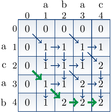
In the figure, the arrows (both regular and thick ones) show the direction(s) which can produce the value mem(i,j). For instance:

The value 2 at mem(4,4) is obtained by taking the value 2 of either mem(3,4) or mem(4,3). This is because $ \LCSa4 \neq \LCSb4 $ and an LCS of $ \LCSAP4 $ and $ \LCSBP4 $ is obtained by taking either (i) an LCS of $ \LCSAP3 $ and $ \LCSBP4 $, or (i) an LCS of $ \LCSAP4 $ and $ \LCSBP3 $.
The value 2 at mem(2,4) is obtained by adding 1 to the value 1 of mem(1,3). This is because $ \LCSa2 = \LCSb4 = b $ and an LCS of $ \LCSAP2 $ and $ \LCSBP4 $ is obtained from an LCS of $ \LCSAP1 $ and $ \LCSBP3 $ by adding $ b $ to it.
The value 1 at mem(1,2) is obtained by taking the value 1 of mem(1,1). This is because $ \LCSa1 \neq \LCSb2 $ and an LCS of $ \LCSAP1 $ and $ \LCSBP1 $ is length 1, which is longer than an length 0 LCS of $ \LCSAP0 $ and $ \LCSBP2 $. Thus one obtains an LCS of $ \LCSAP1 $ and $ \LCSBP2 $ by taking a LCS of $ \LCSAP1 $ and $ \LCSBP1 $.

The thick arrows illustrate the reversed solution construction path. In this particular case, the constructed solution is $ \Seq{a,b} $.

Compare the constructed table to the tree call figure with memoization shown earlier.

The thick path in the table corresponds to the call tree path giving the same solution.
In the tree, only the necessary recursion calls are made.

In the table however, some unnecessary entries such as mem(3,2) above are computed. They do not contribute to any solutions.