Approaches for Solving NP-Complete problems

So what to do when a problem is NP-complete? As there are lots practical problems that have to be solved even though they are NP-complete (or even harder), one has to develop some approaches that work “well enough” in practice. Some alternatives are:

Develop backtracking search algorithms with efficient heuristics and pruning techniques.
Attack some special cases occurring in practice.
Develop approximation algorithms.
Apply incomplete local search methods.
Use existing tools.

Exhaustive search

Perhaps the simplest way to solve computationally harder problems is to exhaustively search through all the solution candidates. This is usually done with a backtracking search that tries to build a solution by extending partial solutions to larger ones. Of course, in the worst case this takes super-polynomial, usually exponential or worse, time for NP-complete and more difficult problems. However, for some instances the search may quickly find a solution or deduce that there is none. The search can usually be improved by adding clever pruning techniques that help detecting earlier that a partial solution cannot be extended to a full solution.

As an example, consider again the subset-sum problem.

Definition: The subset-sum problem

Instance: A set \(S\) of integers and a target value \(t\).

Question: Does \(S\) have a subset \(S' \subseteq S\) such that \(\sum_{s \in S'}s = t\)?

A straightforward recursive backtracking search algorithm for it can be implemened in Scala as follows.

def solve(set: Set[Int], target: Int): Option[Set[Int]] =
  def inner(s: Set[Int], t: Int): Option[Set[Int]] =
    if t == 0 then return Some(Set[Int]())
    else if s.isEmpty then return None
    val e = s.head
    val rest = s - e
    // Search for a solution without e
    val solNotIn = inner(rest, t)
    if solNotIn.nonEmpty then return solNotIn
    // Search for a solution with e
    val solIn = inner(rest, t - e)
    if solIn.nonEmpty then return Some(solIn.get + e)
    // No solution found here, backtrack
    return None
  inner(set, target)

For the instance in which \(S = \Set{-9,-3,7,12}\) and \(t = 10\), the call tree of the above program looks like this:

The search procedure can be improved by adding a pruning rule that detects whether the target value is too large or too small so that the number in the set \(S\) can never sum to it:

def solve(set: Set[Int], target: Int): Option[Set[Int]] =
  def inner(s: Set[Int], t: Int): Option[Set[Int]] =
    if t == 0 then return Some(Set[Int]())
    else if s.isEmpty then return None
    else if s.filter(_ > 0).sum < t || s.filter(_ < 0).sum > t then
      // The positive (negative) numbers cannot add up (down) to t
      return None
    val e = s.head
    val rest = s - e
    // Search for a solution without e
    val solNotIn = inner(rest, t)
    if solNotIn.nonEmpty then return solNotIn
    // Search for a solution with e
    val solIn = inner(rest, t - e)
    if solIn.nonEmpty then return Some(solIn.get + e)
    // No solution found here, backtrack
    return None
  inner(set, target)

Now the call tree for the same instance as above, \(S= \Set{-9,-3,7,12}\) and \(t = 10\), is smaller because some of the search branches get terminated earlier:

Special cases

Sometimes we have a computationally hard problem but the instances that occur in practice are somehow restricted special cases. In such a case, it may be possible to develop an algorithm that solves such special instances efficiently. Technically, we are not solving the original problem anymore but a different problem where the instance set is a subset of the original problem instance set.

Example: subset-sum with smallish values

In the case of subset-sum, one can develop a Dynamic programming algorithm that works very well for “smallish” numbers. First, define a recursive function \(\SSDP(S,t)\) evaluating to true if and only if \(S = \Set{v_1,v_2,...,v_n}\) has a subset that sums to \(t\):

\(\SSDP(S,t) = \True\) if \(t = 0\),
\(\SSDP(S,t) = \False\) if \(S = \emptyset\) and \(t \neq 0\),
\(\SSDP(S,t) = \True\) if \(\SSDP(\Set{v_2,v_3,...,v_n},t)=\True\) or \(\SSDP(\Set{v_2,v_3,...,v_n},t-v_1)=\True\), and
\(\SSDP(S,t) = \False\) otherwise.

Now, using the memoization technique with arrays, it is possible to implement a dynamic programming algorithm that works in time \(\Oh{\Card{S} M}\) and needs \(\Oh{M \log_2 M}\) bytes of memory, where \(M = \sum_{s \in S,s > 0}s - \sum_{s \in S,s < 0}s\) is the size of the range in which the sums of all possible subsets of \(S\) must be included. Solution reconstruction is also quite straightforward. Algorithm sketch:

Take an empty array \(a\).
For each number \(x \in S\) in turn, insert in one pass
- \(a[y+x] = x\) for each \(y\) for which \(a[y]\) is already defined, and
- \(a[x] = x\).

That is, in a number-by-number manner, insert all the subset sums that can be obtained either using the number alone or by adding it to any of the sums obtainable by using earlier numbers. The value written in the element \(a[s]\) tells what was the last number inserted to get the sum \(s\); this allows reconstruction of the solution subset.

Example

Assume that the set of numbers is \(S= \Set{2,7,14,49,98,343,686,2409,2793,16808,17206,117705,117993}\). The beginning of the array is

Inspecting the array, one can directly see that, for instance, there is a subset \(S' \subseteq S\) for which \(\sum_{s \in S'} = 58\) and that such a subset is obtained with the numbers \(a[58] = 49\), \(a[58-49] = a[9] = 7\) and \(a[9-7] = a[2] = 2\).

Is the dynamic programming algorithm above a polynomial time algorithm for the NP-complete problem subset-sum? No, unfortunately it is not:

the size of the input instance is the number of bits needed to represent the numbers, and
therefore the value of the sum \(\sum_{s \in S,s > 0}s - \sum_{s \in S,s < 0}s\), and thus the running time as well, can be exponentially large with respect to the instance size.

For instance, the numbers that were produced in our earlier reduction from 3-CNF SAT to subset-sum are not small: if the 3-CNF SAT instance has \(n\) variables and \(m\) clauses, then the numbers have \(n+m\) digits and their values are in the order \(10^{n+m}\), i.e., exponential in \(n+m\). Note: if the dynamic programming approach is implemented with hash maps instead of arrays, then it works for the special case when the numbers are not necessarily “smallish” but when the number of different sums that can be formed from \(S\) is “smallish”.

Reducing to an another problem

For some NP-complete and harder problems there are some very sophisticated solver tools that work extremely well for many practical instances:

propositional satisfiability: MiniSat, kissat and others
integer linear programming (ILP): lp_solve, SCIP, Google OR-Tools, IBM ILOG CPLEX and others
satisfiability modulo theories: Z3 and others
and many others …

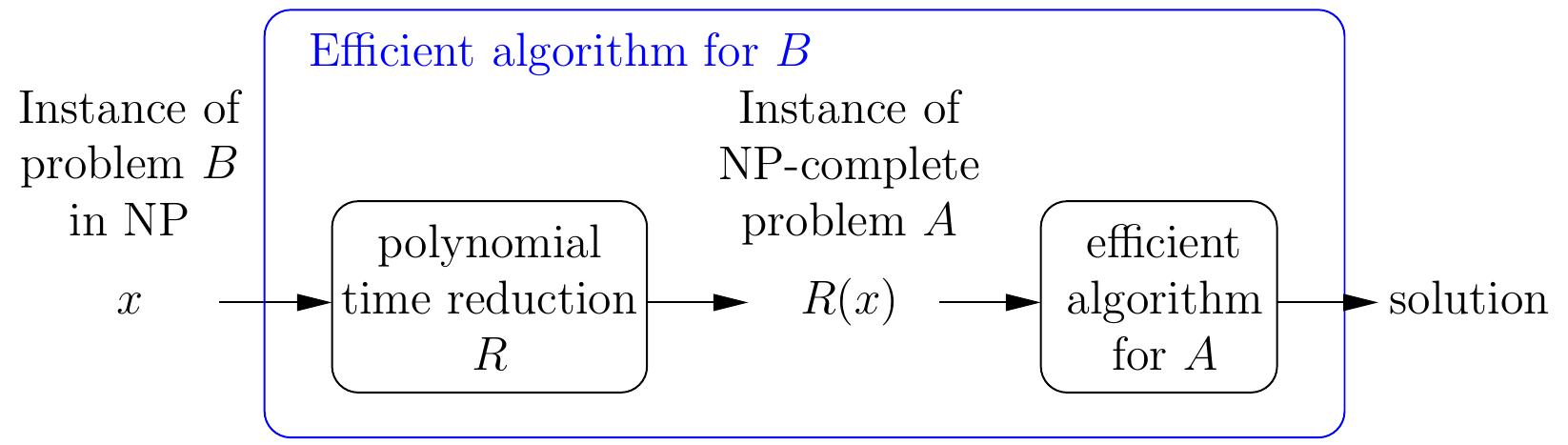
Thus if one can reduce the current problem \(B\) into one of the problems \(A\) above, it may be possible to obtain a practically efficient solving method without programming the search method by one-self. Notice that here we are using reductions in the other direction compared to the case when we proved problems NP-complete: we now take the problem which we would like to solve and reduce it a problem for which we have an usually-efficient tool available.

Example: solving Sudokus with SAT

Let us apply the above described approach to Sudoku solving. Our goal is to use the sophisticated CNF SAT solvers available. Thus, given an \(n \times n\) partially filled Sudoku grid, we want to make a propositional formula \(\phi\) such that

the Sudoku grid has a solution if and only the formula is satisfiable, and
from a satisfying assignment for \(\phi\) we can build a solution for the Sudoku grid.

In practice we thus want to use the following procedure:

To obtain such a CNF formula \(\phi\) for a Sudoku grid, we first introduce a variable

\[\SUD{r}{c}{v}\]

for each row \(r = 1,...,n\), column \(c = 1,...,n\) and value \(v = 1,...,n\). The intuition is that if \(\SUD{r}{c}{v}\) is true, then the grid element at row \(r\) and column \(c\) has the value \(v\). The formula

\[\phi = C_1 \land C_2 \land C_3 \land C_4 \land C_5 \land C_6\]

is built by introducing sets of clauses that enforce different aspects of the solution:

Each entry has at least one value: \(C_1 = \bigwedge_{1 \le r \le n, 1 \le c \le n}(\SUD{r}{c}{1} \lor \SUD{r}{c}{2} \lor ... \lor \SUD{r}{c}{n})\)
Each entry has at most one value: \(C_2 = \bigwedge_{1 \le r \le n, 1 \le c \le n,1 \le v < v' \le n}(\neg\SUD{r}{c}{v} \lor \neg\SUD{r}{c}{v'})\)
Each row has all the numbers: \(C_3 = \bigwedge_{1 \le r \le n, 1 \le v \le n}(\SUD{r}{1}{v} \lor \SUD{r}{2}{v} \lor ... \lor \SUD{r}{n}{v})\)
Each column has all the numbers: \(C_4 = \bigwedge_{1 \le c \le n, 1 \le v \le n}(\SUD{1}{c}{v} \lor \SUD{2}{c}{v} \lor ... \lor \SUD{n}{c}{v})\)
Each block has all the numbers: \(C_5 = \bigwedge_{1 \le r' \le \sqrt{n}, 1 \le c' \le \sqrt{n}, 1 \le v \le n}(\bigvee_{(r,c) \in B_n(r',c')}\SUD{r}{c}{v})\) where \(B_n(r',c') = \Setdef{(r'\sqrt{n}+i,c'\sqrt{n}+j)}{0 \le i < \sqrt{n}, 0 \le j < \sqrt{n}}\)
The solution respects the given cell values \(\SUDHints\): \(C_6 = \bigwedge_{(r,c,v) \in \SUDHints}(\SUD{r}{c}{v})\)

The resulting formula has \(\Card{\SUDHints}\) unary clauses, \(n^2\frac{n(n-1)}{2}\) binary clauses, and \(3n^2\) clauses of length \(n\). Thus the size of the formula is polynomial with respect to \(n\).

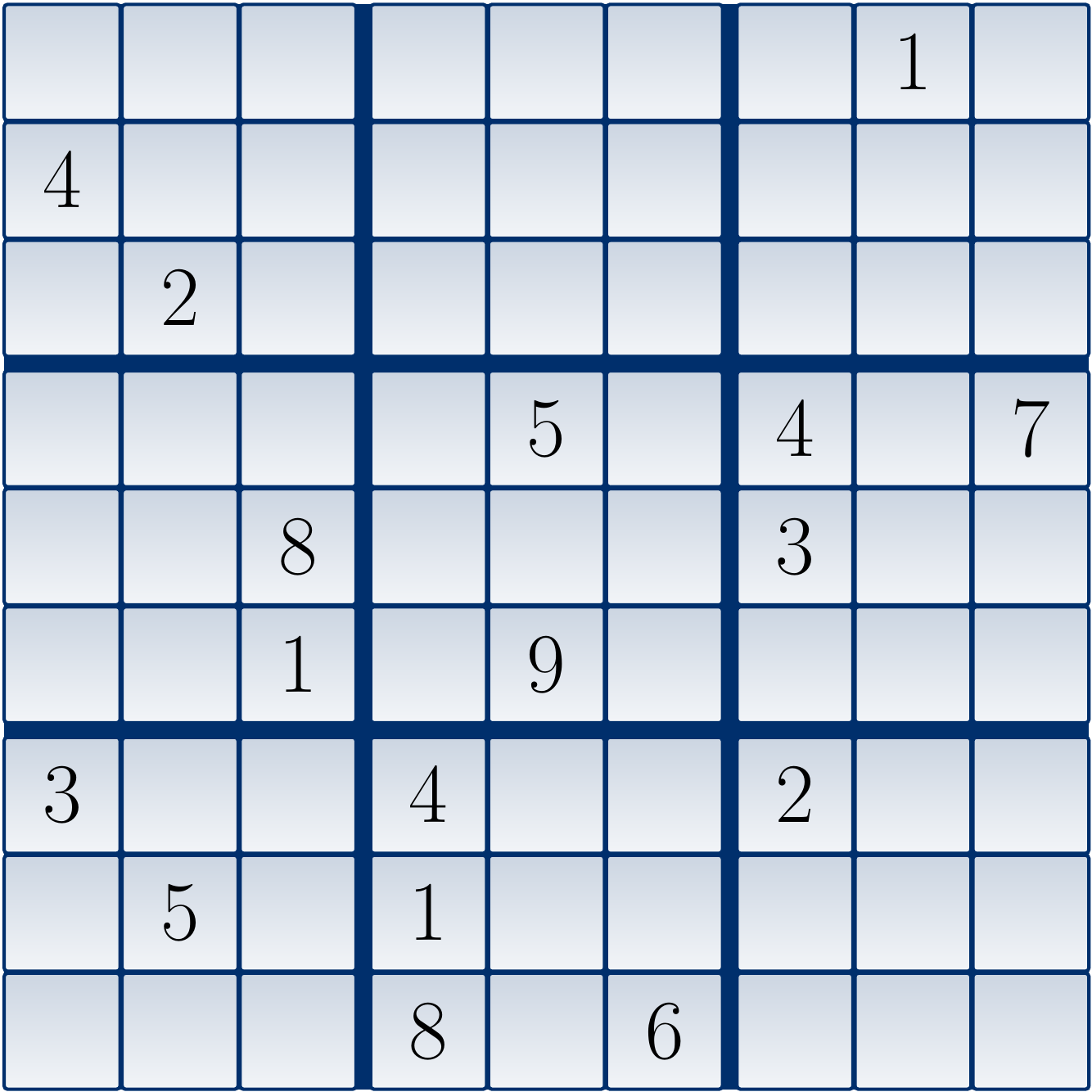
Example

Consider the Sudoku grid below.

The corresponding CNF formula is the following.

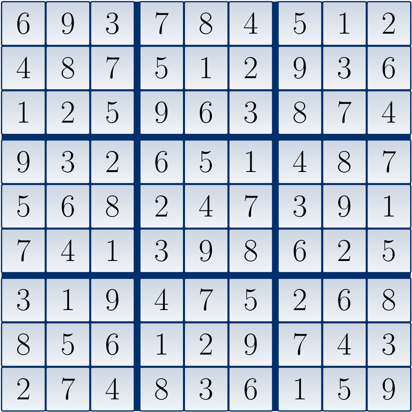
\begin{eqnarray*} (x_{1,1,1} \lor x_{1,1,2} \lor ... \lor x_{1,1,9}) \land ... \land (x_{9,9,1} \lor x_{9,9,2} \lor ... \lor x_{9,9,9}) &\land&\\ (\neg x_{1,1,1} \lor \neg x_{1,1,2}) \land ... \land (\neg x_{9,9,8} \lor \neg x_{9,9,9}) &\land&\\ (x_{1,1,1} \lor x_{1,2,1} \lor ... \lor x_{1,9,1}) \land ... \land (x_{9,1,9} \lor x_{9,2,9} \lor ... \lor x_{9,9,9}) &\land&\\ (x_{1,1,1} \lor x_{2,1,1} \lor ... \lor x_{9,1,1}) \land ... \land (x_{1,9,9} \lor x_{2,9,9} \lor ... \lor x_{9,9,9}) &\land&\\ (x_{1,1,1} \lor x_{1,2,1} \lor ... \lor x_{3,3,1}) \land ... \land (x_{7,7,9} \lor x_{7,8,9} \lor ... \lor x_{9,9,9}) &\land&\\ (x_{1,8,1}) \land (x_{2,1,4}) \land (x_{3,2,2}) \land ... \land (x_{9,6,6})&& \end{eqnarray*}

When the formula is given to a SAT solver, it declares that the formula has a model in which all \(x_{1,1,i}\) except \(x_{1,1,6}\) are false, and so on. From the variables that are true, we obtain the following unique solution to the original Sudoku grid.

An implementation of this approach, using the Sat4j SAT solver implemented in Java, is available in the assignment package of the “coloring with SAT” programming exercise. Feel free to compare its performance to the Sudoku solver you implemented in the CS-A1120 Programming 2 course.

Note

This approach of describing an instance of some other problem as a satisfiability instance, or an instance of some other similar constraint satisfaction formalism, is also called constraint programming.

It is a form of declarative programming: one only declares how the solution should look like, and a constraint solver then finds one (or states that none exists).