$$ $$ $$ $$ $$ $$ $$ $$ $$ $$ $$ $$ $$ $$ $$ $$ $$ $$ $$ $$ $$ $$ $$ $$ $$ $$ $$ $$ $$ $$ $$ $$ $$ $$ $$ $$ $$ $$ $$ $$ $$ $$ $$ $$ $$ $$ $$ $$ $$ $$ $$ $$ $$ $$ $$ $$ $$ $$ $$ $$ $$ $$ $$ $$ $$ $$ $$ $$ $$ $$ $$ $$ $$ $$ $$ $$ $$ $$ $$ $$ $$ $$ $$ $$ $$ $$ $$ $$ $$ $$ $$ $$ $$ $$ $$ $$ $$ $$ $$

$$ $$ $$ $$ $$ $$ $$ $$ $$ $$ $$ $$ $$ $$ $$ $$ $$ $$

$$ $$ $$ $$ $$ $$ $$ $$ $$ $$ $$ $$ $$ $$ $$ $$ $$

$$ $$ $$ $$ $$ $$ $$ $$ $$ $$ $$ $$ $$ $$ $$ $$ $$ $$

Minimum spanning trees

Consider a connected, undirected, and edge-weighted graph $G=(V,E,w)$. A spanning tree of $G$ is a connected acyclic graph $T=(V,A,w)$ with $A\subseteq E$. Its weight is the sum of its edge weights $\sum _{\{u,v\}\in A}w(\{u,v\})$. A spanning tree of $G$ is a minimum spanning tree (MST) of $G$ if its weight is the smallest among all spanning trees of $G$. Observe that a graph can have many minimum spanning trees.

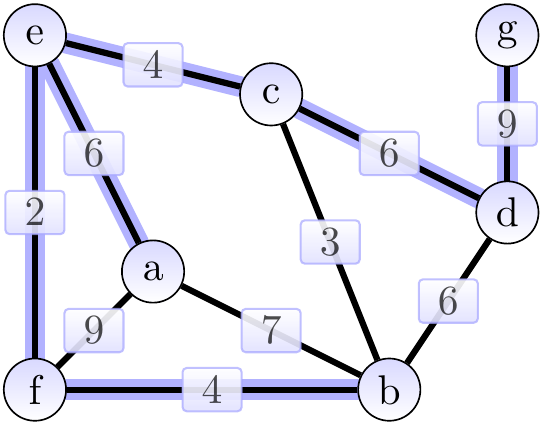
Example

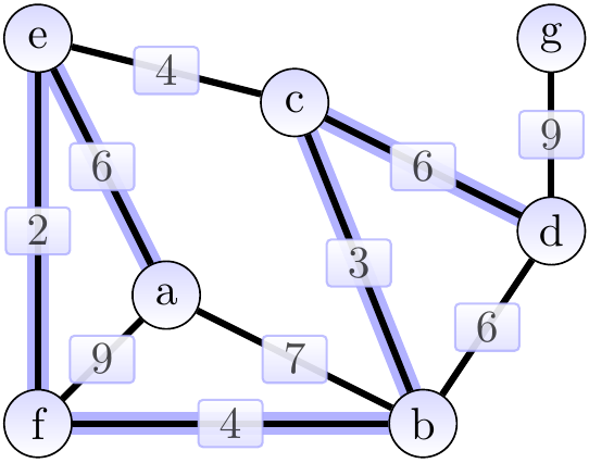
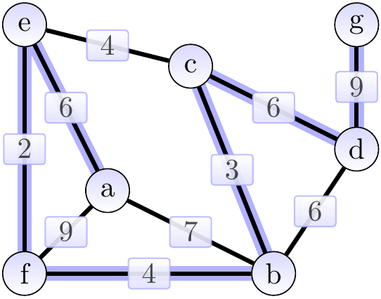
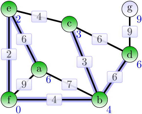
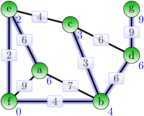
Consider the graph shown below.

The highlighted edges in the two graphs below show two spanning trees for the graph above. The first one has weight 31 and is not minimum. The second one is a minimum spanning tree with weight 30.

As an application example, if the graph models an electronic circuit board so that

• ​ the vertices are the components and

• ​ the edges are the possible routes for the power/clock wires between the components,

then a minimum spanning tree of the graph gives a way to connect all the components with the power/clock wire by using the minimum amount of wire.

Note that we only consider connected graphs: for graphs with many components, we could compute a minimum spanning trees for each component individually. And we only consider edge-weighted undirected graphs; for directed graphs the analog concept is called “spanning arborescence of minimum weight” or “optimal branching”, see, for instance, the Wikipedia page on Edmond’s algorithm. These are not included in the course.

A generic greedy approach

Given a graph, it may have an exponential amount of spanning trees. Thus enumerating over all of them in order to find a minimum one is not a feasible solution. But there are very fast algorithms solving the problem:

• ​ Kruskal’s algorithm

• ​ Prim’s algorithm

Both are greedy algorithms (recall Section Greedy Algorithms). They build an MST by starting from an empty set and then adding edges greedily one-by-one until the edge set is a tree spanning the whole graph. During the construction of this edge set, call it $A$, both maintain the following invariant:

Before each iteration of the main loop, $A$ is a subset of some MST.

To maintain the invariant, the algorithms then select and add a safe edge for $A$: an edge $\{u,v\}\notin A$ such that $A\cup \{\{u,v\}\}$ is also a subset of some MST. Such an edge always exists until $A$ is an MST: as $A$ is a subset of some MST, then there is an edge in that MST but not in $A$ and we can add it to $A$. The greedy heuristics are used to select such a safe edge efficiently. The generic version in pseudo-code:

MST-Generic($G=(V,E,w)$): $A\leftarrow \mathrm{\varnothing }$ // The edges in the MST while $A$ does not form a spanning tree: let $\{u,v\}$ be a safe edge for $A$ $A\leftarrow A\cup \{\{u,v\}\}$ return $A$

We now only need a way to efficiently detect safe edges. For that, we use the following definitions:

• ​ A cut for a graph $G=(V,E,w)$ is a partition $(S,V\setminus S)$ of $V$.

• ​ An edge crosses a cut $(S,V\setminus S)$ if its other endpoint is in $S$ and other in $V\setminus S$.

• ​ An edge is a light edge crossing a cut if its weight is the smallest among those edges that cross the cut.

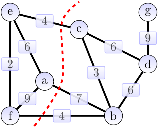
Example

Consider the graph below. The cut $(\{a,e,f\},\{b,c,d,g\})$ is shown with a dashed red line. The edges $\{a,b\}$, $\{b,f\}$ and $\{c,e\}$ cross the cut. The light edges crossing the cut are $\{b,f\}$ and $\{c,e\}$.

The following theorem gives an easy method for the greedy algorithms to select the next safe edge to be included in the MST under construction. Essentially, it says that for any cut that doesn’t split the partial MST under construction, one can choose any crossing edge with the smallest weight to be included in the MST. We need one more definition: a cut $(S,V\setminus S)$ respects a set $A\subseteq E$ of edges if no edge in $A$ crosses the cut.

Theorem

Let $G=(V,E,w)$ be an undirected, connected edge-weighted graph. If $A$ is a subset of an MST for $G$, $(S,V\setminus S)$ is a cut for $G$ that respects $A$ and $\{u,v\}$ is a light edge crossing $(S,V\setminus S)$, then $\{u,v\}$ is a safe edge for $A$.

Example

Again, consider the graph below. The cut $(\{a,e,f\},\{b,c,d,g\})$ is shown with a dashed red line. The edges $\{a,b\}$, $\{b,f\}$ and $\{c,e\}$ cross the cut.

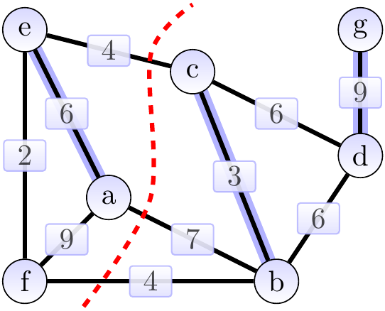
The light edges crossing the cut are $\{b,f\}$ and $\{c,e\}$. The edges in $A$, the MST under construction, are highlighted. They are a subset of an MST. The cut respects $A$. By the theorem, either of the light edges can be added to $A$ so that the result is still a subset of an MST.

Proof: (Sketch)

Let $A^{\prime }$ be the edge set of any MST $T^{\prime }$ such that $A\subset A^{\prime }$ holds.

If $\{u,v\}\in A^{\prime }$, then it is safe for $A$ and we are done.

Suppose that $\{u,v\}\notin A^{\prime }$, $u\in S$, and $v\in V\setminus S$. In the MST $T^{\prime }$ there is a unique simple path from $u$ to $v$ as it is a tree. Let $y$ be the first vertex in this path that belongs to the set $V\setminus S$ and let $x$ be its predecessor in the path still belonging to the set $S$. The edge $\{x,y\}$ does not belong to the set $A$ as the cut respects the edge set. As the edge $\{u,v\}$ is a light edge crossing the cut, it holds that $w(\{u,v\})\le w(\{x,y\})$ as also $\{x,y\}$ crosses the cut. Consider the tree $T$ obtained by first removing the edge $\{x,y\}$ from the tree $T^{\prime }$ (this results in two disjoint trees, other including the vertex $u$ and the other the vertex $v$) and then adding the edge $\{u,v\}$. The weight of this tree $T$ is at most the weight of the tree $T^{\prime }$; as $T^{\prime }$ is minimal, also $T$ is and thus the edge $\{u,v\}$ is safe for $A$.

Kruskal’s algorithm

Kruskal’s algorithm finds the next safe edge to be added by

• ​ first sorting the edges in non-decreasing order by their weight, and

• ​ then finding the smallest-weight edge that connects two trees in the current edge set $A$.

To quickly detect whether an edge connects two trees, the vertices in the trees are maintained in a disjoint-sets data structure (recall Section Disjoint-sets with the union-find data structure). When an edge is added, the trees in question merge into a new larger tree. The cut is not explicitly maintained but for an edge $\{u,v\}$ connecting two trees involving $u$ and $v$ respectively, one can take any cut that puts the tree of $u$ on one side and the tree of $v$ to the other. The possible other trees are put on either side.

In pseudo-code:

MST-Kruskal($Q=(V,E,w)$): $A\leftarrow \mathrm{\varnothing }$ for each vertex $v\in V$: // All vertices are initially in their own unit sets $\mathsf{\text{make-set}}(v)$ sort the edges $E$ into nondecreasing order by their weight for each edge $\{u,v\}\in E$ in nondecreasing weight-order: if $\mathsf{\text{find-set}}(u)\ne \mathsf{\text{find-set}}(v)$: // Are $u$ and $v$ in different sets? $A\leftarrow A\cup \{\{u,v\}\}$ // Record the merge edge $\mathsf{\text{union}}(u,v)$ // Merge the sets return $A$

With the rank-based disjoint-sets implementation introduced in Section Disjoint-sets with the union-find data structure, one can argue that the worst-case running time of the algorithm is $O(|E|{\log }_2|E|)$ — sorting the edges takes asymptotically the largest amount of time in the algorithm. Recalling that $|E|\le {|V|}^2$ and thus ${\log }_2|E|\le 2{\log }_2|V|$, the worst-case bound can be stated also as $O(|E|{\log }_2|V|)$.

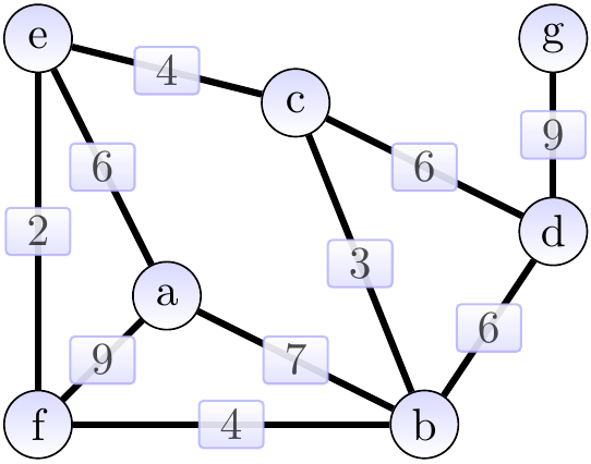
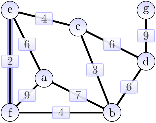
Example: Applying Kruskal’s algorithm

Consider the graph shown below. The edges in a weight-sorted order are (edges with the same weight are ordered arbitrarily): $\{e,f\},\{b,c\},\{b,f\},\{c,e\},\{c,d\},\{a,e\},\{b,d\},\{a,b\},\{a,f\},\{d,g\}$.

First, we add the edge $\{e,f\}$ of weight 2 and obtain the situation below (the edges in the MST under construction $A$ are highlighted). The cut considered could be $(\{e\},\{a,b,c,d,f,g\})$.

Next, we add the edge $\{b,c\}$ of weight 3 and obtain the situation below. The cut considered could be $(\{b\},\{a,c,d,e,f,g\})$.

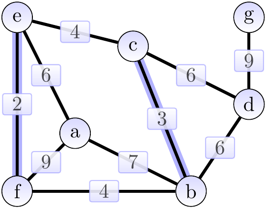
Next, we add the edge $\{b,f\}$ of weight 4 and obtain the situation below. The cut considered could be $(\{e,f\},\{a,b,c,d,g\})$.

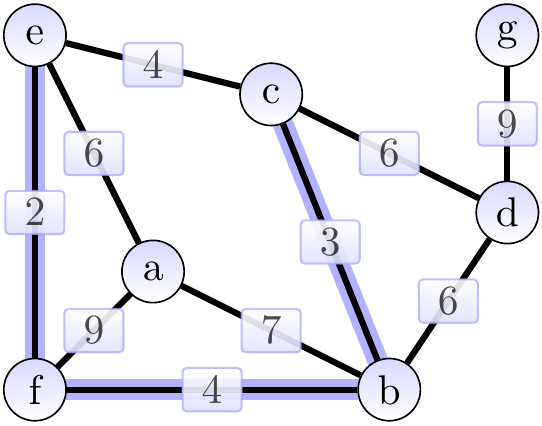
The next edge $\{c,e\}$ is skipped because the vertices $c$ and $e$ already belong to the same tree. After this, we add the edge $\{c,d\}$ of weight 6 and obtain the situation below. The cut considered could be $(\{b,c,e,f\},\{a,d,g\})$.

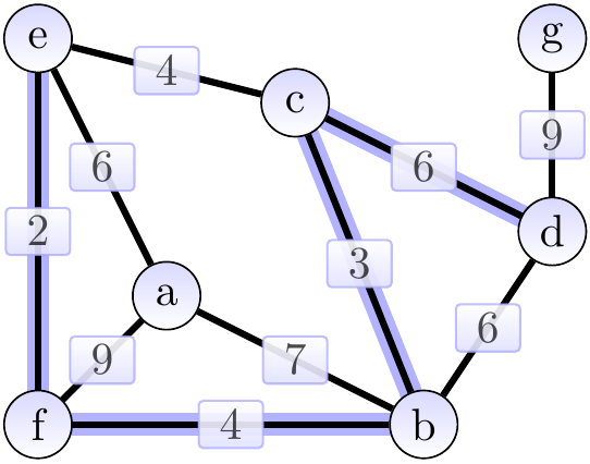
Next, we add the edge $\{a,e\}$ of weight 6 and obtain the situation below. The cut considered could be $(\{a\},\{b,c,d,e,f,g\})$.

The next edges $\{b,d\}$, $\{a,b\}$, and $\{a,f\}$ are skipped because their end-points already belong to the same tree. Finally, we add the edge $\{d,g\}$ of weight 9 and obtain the situation below. The cut considered could be $(\{a,b,c,d,e,f\},\{g\})$.

The result shown above is an MST of weight 30.

Prim’s algorithm

Prim’s algorithm also implements the generic greedy MST finding algorithm but selects the next safe edge in a different way. It maintains the cut explicitly:

• ​ on the other half is the whole MST constructed so far, while

• ​ the other half are the vertices not yet joined to the MST.

The process starts from an arbitrary root vertex. Then, at each step, an arbitrary light edge from the first half to the second half is selected and thus one vertex is moved from the second half to the first. To select a light edge quickly, each vertex in the second half maintains, as attributes, the weight (referred to as “key” in the pseudo-code) and the other end of a smallest weight edge (“parent” in the pseudo-code) coming to it from the first half. All the vertices in the second half are stored in a minimum priority queue $Q$ (recall Section Priority queues with binary heaps) with the weight acting as the priority key. In this way, it is efficient to find the vertex with the smallest key: the edge from the first half to it must thus be a light edge. In the beginning, all the weights are $\mathrm{\infty }$ except for the root vertex which has weight 0. Whenever a vertex is moved from the second half to the first (dequeued from the priority queue), its neighbors’ attributes are updated.

In pseudo-code:

MST-Prim($G=(V,E,w)$, $\mathit{root}$): for each vertex $v\in V$: $v.\mathsf{\text{key}}\leftarrow \mathrm{\infty }$ $v.\mathsf{\text{parent}}\leftarrow \mathbf{\text{nil}}$ $\mathit{root}.\mathsf{\text{key}}=0$ $Q\leftarrow V$ // Min-priority queue (w.r.t. the key) of the vertices not yet in the MST $A\leftarrow \mathrm{\varnothing }$ // The edges in the MST while $Q\ne \mathrm{\varnothing }$: let $u$ be a vertex in $Q$ with the smallest key remove $u$ from $Q$ if $u\ne \mathit{root}$: $A\leftarrow A\cup \{\{u.\mathsf{\text{parent}},u\}\}$ for each vertex $v$ with an edge $\{u,v\}\in E$: if $v\in Q$ and $w(\{u,v\})<v.\mathsf{\text{key}}$: $v.\mathsf{\text{parent}}\leftarrow u$ $v.\mathsf{\text{key}}\leftarrow w(\{u,v\})$ return $A$

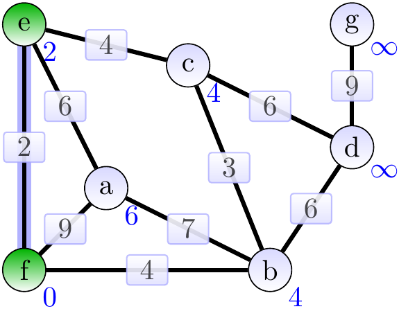
Example: Applying Prim’s algorithm

Consider again the graph shown below.

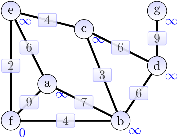
The graphs below show the constructed spanning tree (the highlighted edges) at the end of each while-loop execution, green vertices are the ones not in $Q$. Supposing that the root vertex was $f$, the situation after the first iteration is shown below. Observe that the weights of the neighbors of $f$ have been updated. The “parent” attributes are not shown in the graph.

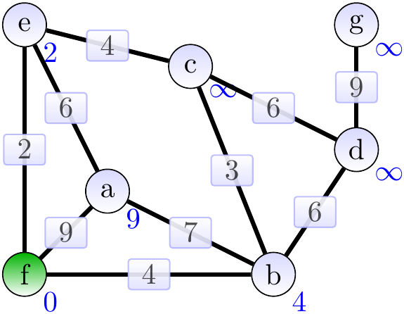
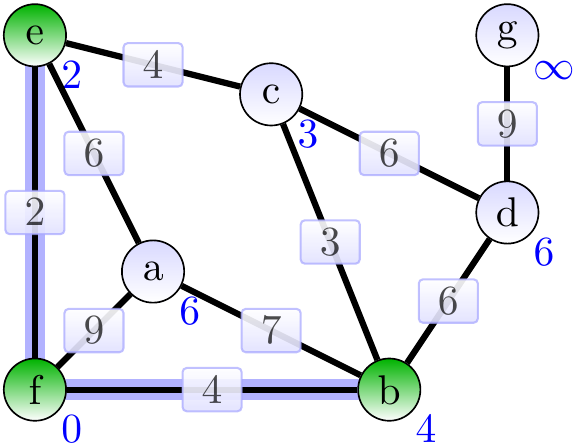
Next, the vertex $e$ with the lowest priority and the edge $\{e,f\}$ are added to the MST. The weights of the neighbors of $e$ are updated.

Now the edge $\{b,f\}$ is added to the MST. Observe that the edge $\{c,e\}$ could have been selected instead and this would result in a different final MST.

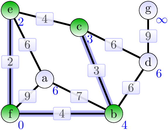
Next, add the edge $\{b,c\}$.

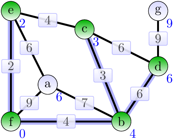
Next, add the adage $\{b,d\}$.

Next, add the age $\{a,e\}$.

Next, add the age $\{d,g\}$.

The final result is an MST of wight 30.

Let’s perform a worst-case running time analysis of the algorithm. Assume that priority queues are are implemented with heaps (recall Section Priority queues with binary heaps).

• ​ The initialization phase, including the priority queue initialization, can be done in $O(|V|{\log }_2|V|)$. It is quite easy to see that in this case it is easy to initialize the priority queue in linear time as well and thus the initialization phase can in fact be done in time $O(|V|)$.

• ​ The while-loop executes $|V|$ times as one vertex is removed from $Q$ in each iteration.

  • ​ Removing a smallest element from the priority queue takes time $O({\log }_2|V|)$

  • ​ The set $A$ can be implemented as a linked list or an array of $|V|-1$ elements and thus adding an edge to it takes constant time.

• ​ Each edge is considered twice, once for each end point

  • ​ The keys of the vertices are thus updates at most $2|E|$ times, each update taking $O({\log }_2|V|)$ time.

The total running time is thus $O(|V|+|V|{\log }_2|V|+|E|{\log }_2|V|)$. This equals to

$$O(|E|{\log }_2|V|)$$

as $|E|\ge |V|-1$ for connected graphs.

A small side track: Steiner trees

As shown above, we have very efficient algorithms for finding minimum spanning trees. But if we make a rather small modification in the problem definition, we obtain a problem for which we do not know any polynomial time algorithms at the moment. In fact, many believe (but we cannot yet prove this) that such algorithms do not exist. Consider the problem of finding minimum Steiner trees instead of minimum spanning trees.

Definition: Minimum Steiner tree problem

Given a connected, edge-weighted undirected graph $G=(V,E,w)$ and a subset $S\subseteq V$ of terminal vertices, find an acyclic sub-graph $G=(V,A,w)$ with $A\subseteq E$ that (i) connects all the terminal vertices to each other with some paths and (ii) minimizes the edge-weight sum $\sum _{\{u,v\}\in A}w(\{u,w\})$.

That is, the tree does not have to span all the vertices but only the terminals and some of the other needed to connect the terminals to each other.

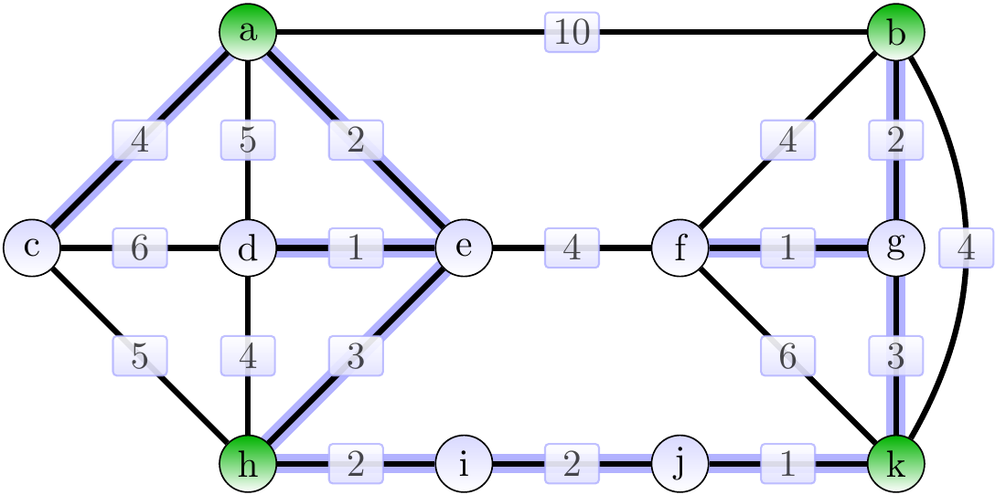
Example

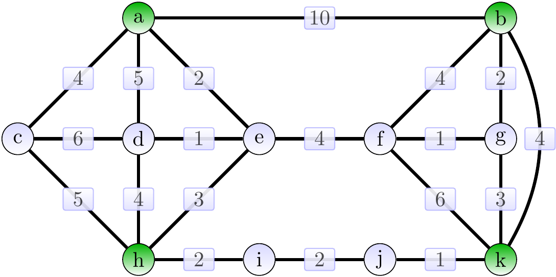
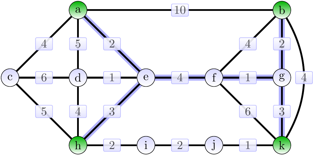
Consider the graph on the left below with the terminal vertices $\{a,b,h,k\}$ shown in green.

The following is a Steiner tree of weight 15.

The graph below shows, in order to illustrate the difference in the problem definition, a minimum spanning tree for the graph.

As an application example, we could extend our earlier circuit board example. Now

• ​ the terminal vertices are the components,

• ​ the other vertices are crossing positions on the board through which we can draw the power/clock wires, and

• ​ the edges are the possible connections between the components and crossings.

We now want to find a minimum Steiner tree instead of a minimum spanning tree as we do not need to connect power/clock wire to each of the crossings, only the components need to be connected to each other.

Finding minimum Steiner trees is one example of an NP-hard problem. For such problems, we do not know algorithms that would have polynomial worst-case running time. There are algorithms that solve the minimum Steiner tree problem in time that is (i) exponential in the size of the terminal set $S$ but (ii) polynomial in the size of the graph. Thus the problem is “fixed-parameter tractable”; see, for instance, this slide set. These algorithms and concepts are not included in the course exam.