Depth-first search

Depth-first search is another systematic method for traversing graphs. Like Breadth-first search, it finds all the vertices that are reachable from the given source vertex. However, it does not necessarily find the shortest paths or the smallest distances from the source vertex. Instead, it can reveal some structure of the graph that can be used in other algorithms (see, for instance, Topological sort and Strongly Connected Components). The idea of the basic version is as follows:

Start visiting vertices from the source vertex.
Recursively visit the white neighbors of the current vertex. When starting the visit, color the vertex gray. When all the neighbors have been (recursively) visited, color the vertex black.

In pseudocode:

Depth-first-search(\(G\), \(s\)):
  for each vertex \(\Vtx \in \Verts\):
    \(\GColor{\Vtx} \Asgn \GWhite\)
    \(\GPred{\Vtx} \Asgn \GNil\)
  def visit(\(u\)):
    \(\GColor{u} \Asgn \GGray\)
    for each \(\Vtx\) with \(\Set{u,\Vtx} \in \Edges\):
      if \(\GColor{\Vtx} = \GWhite\):
        \(\GPred{\Vtx} \Asgn u\)
        visit(\(\Vtx\))
    \(\GColor{u} \Asgn \GBlack\)
  visit(\(s\))

Example: Depth-first search on an undirected graph

The animation below shows a depth-first search on an undirected graph. The figures show the situation at the beginning and end of each call to the visit function (the currently visited node is shown in blue) and at the end of the algorithm (the last figure). The neighbors of a vertex are visited in alphabetic order.

Again, for directed graphs one just replaces the line “for each \(\Vtx\) with \(\Set{u,\Vtx} \in \Edges\)” with “for each \(\Vtx\) with \(\Tuple{u,\Vtx} \in \Edges\)”.

Example: Depth-first search on a directed graph

Worst-case running time analysis of the algorithm:

Each vertex is visited once (it must be white to be visited and immediately turns gray when visited).
While a vertex is visited, each edge from it is traversed.

Therefore, the algorithm runs in linear time \(\Oh{\Card{\Verts}+\Card{\Edges}}\).

Observe that the (reversed) predecessor links give a path, but not necessarily a shortest one, from the source vertex to each vertex reachable from the source.

An extended version

Let us extend the basic version by attaching to each vertex two visit timestamp attributes:

the start timestamp tells the “time” on which visiting the vertex started (the vertex was colored to gray), and
the finish timestamp tells the time when visiting the vertex was completed (the vertex was colored to black).

The timestamps are ascending integers starting from 1. In addition to the timestamps, the algorithm is extended so that there is no single source vertex for the search but new source vertices are taken (arbitrarily or with some strategy) for sub-searches until all the vertices have been visited. The algorithm now does not find the vertices reachable from a single source vertex but reveals some structure of the graph. In pseudocode, the extended version is:

Depth-first-search(\(G = \Tuple{\Verts,\Edges}\)):
  for each vertex \(\Vtx \in \Verts\):
    \(\GColor{\Vtx} \Asgn \GWhite\)
    \(\GPred{\Vtx} \Asgn \GNil\)
  \(\GTime \Asgn 0\)

  def visit(\(u\)): // Inner recursive function for traversing vertices
    \(\GTime \Asgn \GTime + 1\)
    \(\GStart{u} = \GTime\)
    \(\GColor{u} \Asgn \GGray\)
    for each \(\Vtx\) with \(\Set{u,\Vtx} \in \Edges\): // \(\Tuple{u,\Vtx} \in \Edges\) for directed graphs
      if \(\GColor{\Vtx} = \GWhite\):
        \(\GPred{\Vtx} \Asgn u\)
        visit(\(\Vtx\))
    \(\GColor{u} \Asgn \GBlack\)
    \(\GTime \Asgn \GTime + 1\)
    \(\GFinish{u} = \GTime\)

  for each vertex \(u \in \Verts\):
    if \(\GColor{u} = \GWhite\):
      visit(\(u\))

Example

Consider the directed graph shown below.

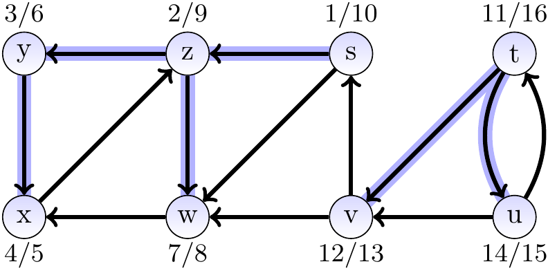
The sub-searches (calls to the visit function in the last line of the main procedure) start from the vertices in alphabetical order in this example so that the first visited vertex is \(s\). Again, the edges from a vertices are traversed in an arbitrary order. The pair \(a/b\) next to a vertex tells the start \(a\) and finish \(b\) timestamp of the vertex.

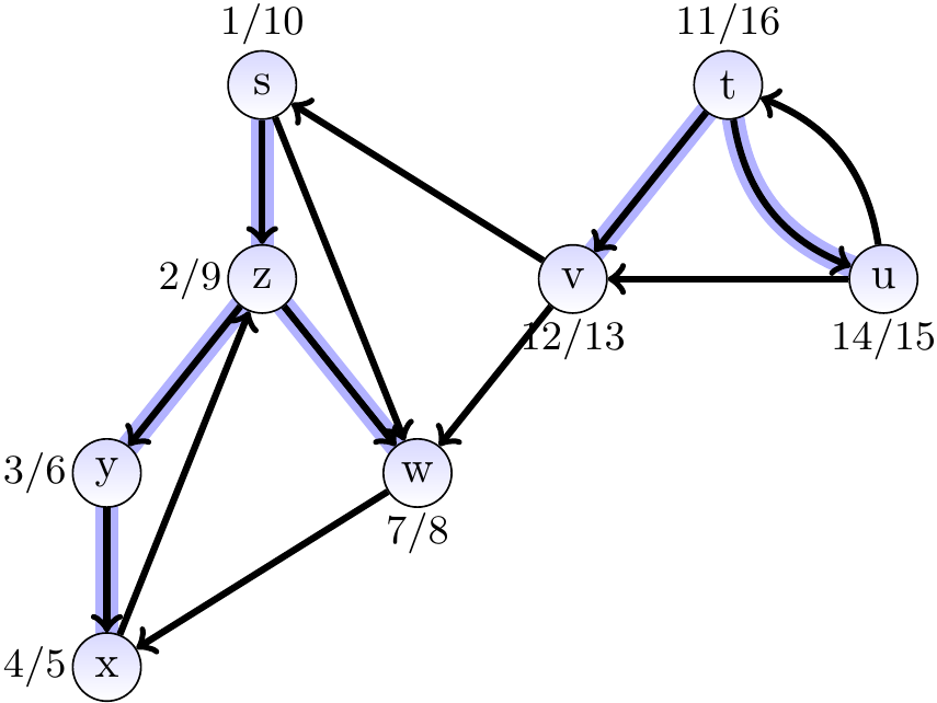
In order to emphasize the traversing order, the same graph is given below but this time drawn differently:

The edges coming from the predecessor vertices form a depth-first forest. Formally, it is the sub-graph \(\GraphP = \Tuple{\Verts,\EdgesP}\), where \(\EdgesP = \Setdef{\Tuple{\GPred{u},u}}{u \in \Verts\text{ and }\GPred{u} \neq \GNil}\). The depth-first forest can consist of several depth-first trees rooted at the vertex first visited in each sub-search. The depth-first forest is not necessarily unique for the graph but depends on traversal order of the depth-first search. Consider the “time interval” \([\GStart{u},\GFinish{u}]\) formed by the timestamps associated to each vertex. For the intervals of two disjoint vertices \(u\) and \(v\) one of the following holds:

\([\GStart{u},\GFinish{u}]\) and \([\GStart{v},\GFinish{v}]\) do not intersect each other (\(u\) and \(v\) belong to different depth-first trees in the forest or are in different branches in the same depth-first tree),
\([\GStart{u},\GFinish{u}]\) is fully contained in \([\GStart{v},\GFinish{v}]\) (\(u\) is a descendant of \(v\) in a depth-first tree), or
\([\GStart{v},\GFinish{v}]\) is fully contained in \([\GStart{u},\GFinish{u}]\) (\(v\) is a descendant of \(u\) in a depth-first tree).

Example

Consider again the directed graph below. Again, the edges in the depth-first forest are highlighted in blue.

The vertices \(z\), \(y\), \(x\) and \(w\) can be reached from \(s\) in the depth-first forest and their time intervals are fully contained in the interval of \(s\).
The intervals of the vertices \(t\), \(v\) and \(u\) belonging to a different depth-first tree do not overlap with the interval of \(s\).

index:: depth-first search: tree edge index:: depth-first search: back edge index:: depth-first search: forward edge index:: depth-first search: cross edge

Assume that a depth-first search has been performed on a directed graph. The edges of the graph can be classified according to the search as follows:

Tree edges are the edges belonging to the depth-first forest.
Back edges are the edges that lead from a vertex to some ancestor vertex in the same depth-first tree (this includes loop-edges).
Forward edges are the edges that lead from a vertex to some proper descendant vertex in the same depth-first tree.
Cross edges are the rest of the edges.

For undirected graphs,

back and forward edges are usually considered to be the same thing, and
there are no cross edges.

Example

Consider the directed graph and depth-first search forest shown below.

The tree edges are highlighted in blue.
The back edges are: \(\Tuple{x,z}\) and \(\Tuple{u,t}\).
The forward edges are: \(\Tuple{s,w}\)
The cross edges are: \(\Tuple{u,v}\), \(\Tuple{v,s}\), \(\Tuple{v,w}\) and \(\Tuple{w,x}\).

Some of the edge types are easy to detect during the depth-first search. Namely, if the algorithm is in the function invocation visit(\(u\)) and considers the edge \(\Tuple{u,\Vtx} \in \Edges\), then that edge is

a tree edge if \(\Vtx\) is white,
a back edge if \(\Vtx\) is gray, and
either a forward or a cross edge if \(\Vtx\) is black.

A directed graph is acyclic if and only if (any) depth-first forest does not contain back edges. As a consequence, the acyclicity of a directed graph can be detected in linear time \(\Oh{\Card{\Verts}+\Card{\Edges}}\).