Numeric integration
In numeric integration, one aims to compute (an approximate) solution of a definite integral. One of the simplest method is to use the trapezoidal rule. With it a definite integral \(\int_a^b f(x) dx\) is approximated by computing the sum
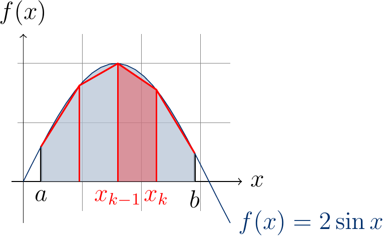
where \(N > 0\) and \(x_k = a + \frac{k}{N}(b - a)\). That is, the interval \([a,b]\) is divided into \(N\) sub-intervals \([x_{k-1},x_k]\) and for each sub-interval the area \(\int_{x_{k-1}}^{x_k}f(x) dx\) is approximated with the formula \((x_k - x_{k-1})\frac{f(x_{k-1}) + f(x_k)}{2}\).
The example figure below shows the approximation of \(\int_{0.3}^{2.9} 2\sin(x) dx\) (the area shaded in blue) when \(N=4\): the approximating area of the sub-interval \([x_2,x_3]\) is shaded in red.

The larger the number \(N\) of sub-intervals is, the better is the approximation. Of course, if the method is applied in some safety-critical application, one should also take into account the precision of the numeric data type used in the implementation (32-bit floats, 64-bit doubles or something else).
Computing the sum is an embarrassingly parallel problem as each sub-interval area approximation \((x_k - x_{k-1})\frac{f(x_{k-1}) + f(x_k)}{2}\) can be computed independently in parallel. The Scala implementation methods below are as follows:
integrate: the sequential reference version,
integratePar1: a straightforward but not so successful attempt to parallelize with.par,map, andsum, and
integratePar2: parallelization by dividing the sum index set \([1..N]\) into \(128 P\) sub-sets, where \(P\) is the number of available CPU cores, and then computing the sum for each sub-set in parallel. The amount \(128 P\) is heuristically selected instead of \(P\) so that if one thread gets interrupted because some other process is scheduled to run, the overall computation can proceed in other sub-sets. Observe that computing the final sum is not parallelized; with current multicore machines, \(P\) is small and the time of computing the sum of \(128 P\) values is negligible compared to the other computations.
// A helper to sum over a sub-interval [start..end] of indices [1..n]
def integrateInterval(f: Double => Double,
		      a: Double, b: Double,
		      start: Int, end: Int,
		      n: Int): Double =
  require(1 <= start && start <= end && end <= n)
  val range = b - a
  var xPrev = a + (start-1) * range / n
  var fPrev = f(xPrev)
  var sum: Double = 0.0
  var i = start
  while i <= end do
    val xCurrent = a + i * range / n
    var fCurrent = f(xCurrent)
    sum += (xCurrent - xPrev) * (fPrev + fCurrent) / 2
    xPrev = xCurrent
    fPrev = fCurrent
    i += 1
  sum

def integrate(f: Double => Double, a: Double, b: Double, n: Int): Double =
  require(a <= b && n > 0)
  integrateInterval(f, a, b, 1, n, n)

def integratePar1(f: Double => Double, a: Double, b: Double, n: Int): Double =
  require(a <= b && n > 0)
  val range = b - a
  (1 to n).par.map(i => {
    val xPrev = a + (i - 1) * range / n
    val xCurr = a + i * range / n
    (xCurr - xPrev) * (f(xPrev) + f(xCurr)) / 2
  }).sum

def integratePar2(f: Double => Double, a: Double, b: Double, n: Int = defaultNofSteps): Double =
  require(a <= b && n > 0)
  val p = Runtime.getRuntime.availableProcessors
  val nofTasks = n min 128*p
  (1 to nofTasks).par.map(t => {
    val start = ((n.toLong * (t-1)) / nofTasks).toInt + 1
    val end = ((n.toLong * t) / nofTasks).toInt
    integrateInterval(f, a, b, start, end, n)
  }).sum
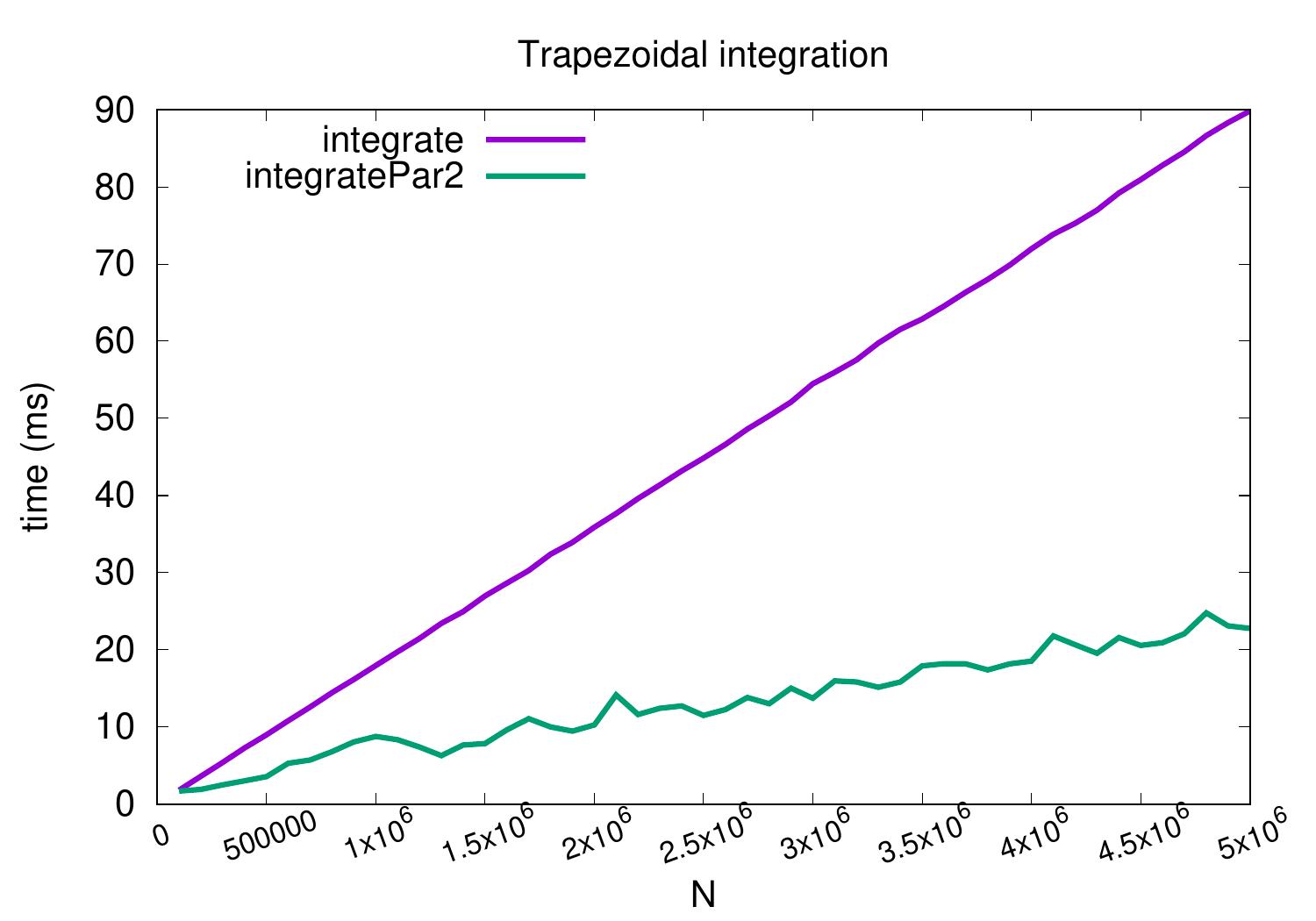
The plot below shows the running times of different methods when computing \(\int_0^1 \sqrt{1-x^2} dx\) for different values of \(N\). The results are obtained on a desktop machine with a quad-core Intel i5-2400 processor running at 3.1 GHz and Scala version 3.1.3.

The method integratePar1 is not included in the plot because it is
slower than the sequential version:
the map method probably builds an intermediate representation over which the final sum is then computed.
It also has to compute the \(x_k\) and \(f(x_k)\) values twice for each \(k\) while
the others are iterative and compute the values only once for most of the indices.
The parallel version integratePar2
obtains a near-linear speedup of roughly 3.7 when \(N = 5 000 000\).