Round 10: Computationally more difficult problems¶

Material:

These notes
Chapter 34 in Introduction to Algorithms, 3rd ed. (online via Aalto lib) on the abstraction level of these notes:
- the formal language definitions are not required,
- nor are the proofs that are not in the notes.

So far almost all of our algorithms have been rather efficient, having worst-case running times such as $ \Oh{\Lg{n}} $, $ \Oh{n} $, $ \Oh{n \Lg{n}} $, $ \Oh{(\NofE + \NofV)\Lg\NofV} $ and so on. But there are lots of (practical!) problems for which we do not know any efficient algorithms. In fact, there are even problems that provably cannot be solved by computers. Here “solve by computers” means “to have an algorithm that in all the cases gives the answer and the answer is correct”. The proof that such problems exists and more about this topic can be found in the Aalto course CS-C2150 Theoretical Computer Science (5cr, periods III-IV).

Example

There is no algorithm that always decides whether a multivariate polynomial has integer-valued roots.

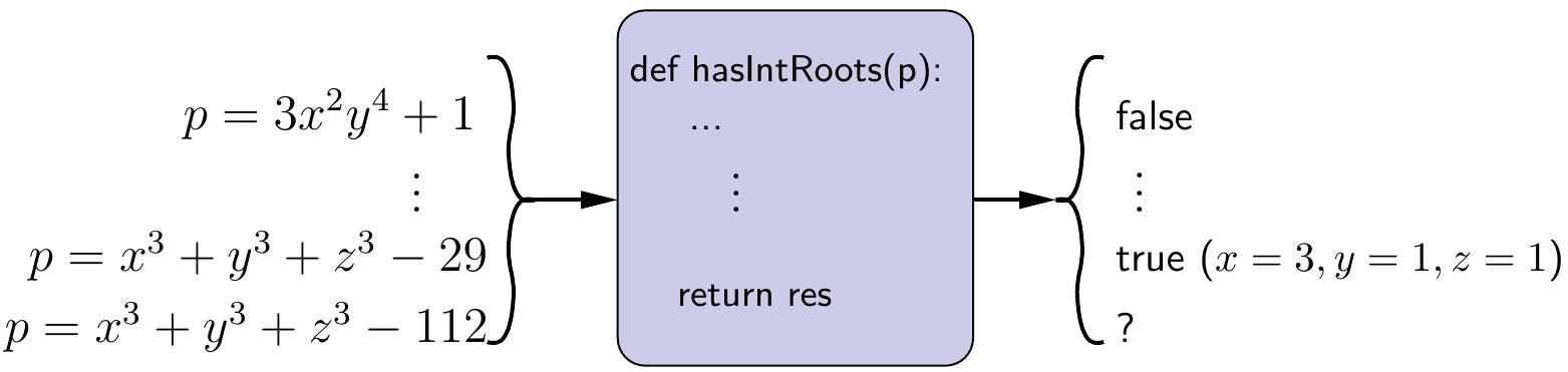
As a curiosity, the output to $ x^3+y^3+z^3-112 $ is marked with “?” in the figure because we do not currently (September 23, 2019) know whether the are integers $ x $, $ y $ and $ z $ such that $ x^3+y^3+z^3 = 112 $. The cases 33 and 42 were solved only in 2019, see this wikipedia article.

This round

gives a semi-formal description for one important class of computationally hard but still solvable problems, called $ \NP $-complete problems, and
provides some methods for attacking such problems in practise.

Definitions by using formal languages etc and most of the proofs are not covered, they are discussed more in the Aalto courses

CS-C2150 Theoretical Computer Science, and
CS-E4530 Computational Complexity Theory.

Computational problems¶

A computational problem consists of a description of what the possible inputs, called instances of the problem, are and what is the question that should be answered on such inputs. As an example, the problem of testing whether an integer is a prime number can be expressed as the following computational problem.

Definition: $ \Prob{Primality} $ problem

Instance: A positive integer $ x $.

Question: Is $ x $ a prime number?

To solve this problem, one has to develop an algorithm that gives the correct answer for all possible input instances.

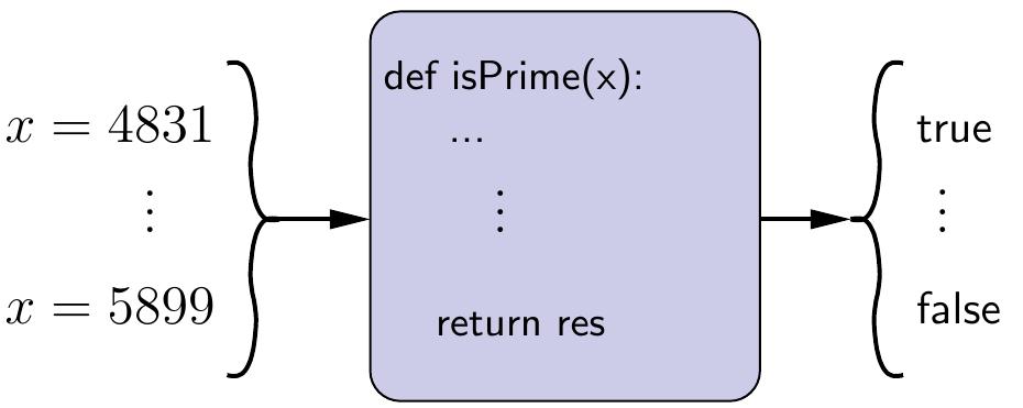
A problem is decidable (or “computable”, or sometimes “recursive” due to historical reasons) if there is an algorithm that can, for all possible instances, answer the question. For instance, the $ \Prob{Primality} $ problem is decidable; a simple but inefficient way to test whether $ x $ is a prime number is to check, for all integers $ i \in [2..\lfloor\sqrt{x}\rfloor] $, that $ i $ does not divide $ x $.

In a decision problem the answer is either “no” or “yes”.

Definition: The $ \SUBSETSUM $ problem

Instance: A set $ S $ of integers and a target value $ t $.

Question: Does $ S $ have a subset $ S’ \subseteq S $ such that $ \sum_{s \in S’}s = t $?

In a function problem the answer is either

“no” when there is no solution, and
a solution when at least one exists.

Definition: The $ \SUBSETSUM $ problem (function version)

Instance: A set $ S $ of integers and a target value $ t $.

Question: Give a subset $ S’ \subseteq S $ such that $ \sum_{s \in S’}s = t $ if such exists.

Mathematically, a computational problem with a no/yes answer can be defined as the set of input strings for which the answer is “yes”. Problems with a more complex answers can be defined as (partial) functions. These formal aspects will be studied more in the Aalto course “CS-C2150 Theoretical computer science”.

In optimization problems one has to find an/the optimal solution.

Definition: $ \MST $ problem

Instance: A connected edge-weighted and undirected graph $ G $.

Question: Give a minimum spanning tree of the graph.

For an optimization problem there usually is a corresponding decision problem with some threshold value for the solution (is there an “at least this good solution”?).

Definition: $ \MSTDEC $ problem

Instance: A connected edge-weighted and undirected graph $ G $ and an integer $ k $.

Question: Does the graph have a spanning tree of weight $ k $ or less?

The full optimization problem is at least as hard as this decision version because an optimal solution gives immediately the solution for the decision version as well.

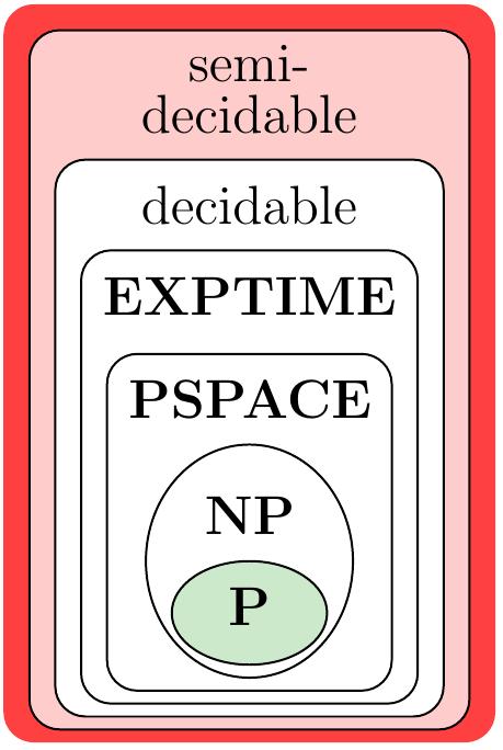
In computational complexity theory, the set of decidable problems can be divided in many smaller complexity classes:

$ \Poly $ — problems that can be solved in polynomial time ($ \approx $ always efficiently) with algorithms
$ \NP $ — problems whose solution can be verified in polynomial time (or that can solved with non-deterministic machines in polynomial time)
$ \PSPACE $ — problems that can be solved with a polynomial amount of extra space (possibly in exponential time)
$ \EXPTIME $ — problems that can be solved in exponential time
and many more…

Polynomial-time solvable problems¶

A problem is polynomial-time solvable if there is an algorithm that solves the problem in time $ \Oh{n^c} $ for some constant $ c $, where $ n $ is the length of the input instance in bits (or, equivalently, in bytes). We consider such problems to be efficiently solvable, or tractable. If a problem is not tractable, then it is intractable. The class of all decision problems that can be solved in polynomial time is denoted by $ \Poly $.

Note

Polynomial-time algorithms involve algorithms with running times such as $ \Theta(n^{100}) $. Such algorithms can hardly be considered as “efficient”. But such running times do not occur often and once a polynomial-time algorithm is found, it is in many cases further improved to run in polynomial-time with a quite small polynomial degree.

Based on the sorting algorithms round, we know how to sort an array of $ n $ elements in time $ \Oh{n \Lg n} $. Thus the following function problem can be solved in polynomial time:

Definition: $ \Prob{median of an array} $ problem

Instance: A sequence of integers.

Question: What is the median of the values in the sequence (“no” if the sequence is empty)?

… and the following decision version is in the class $ \Poly $:

Definition: $ \Prob{median of an array (a decision version)} $ problem

Instance: A sequence of integers and an integer $ k $.

Question: Is the median of the values in the sequence $ k $ or more?

From the graph rounds we know how to efficiently compute shortest paths between the vertices in a graph. Thus the following problem belongs to $ \Poly $:

Definition: $ \Prob{shortest path} $ problem

Instance: an undirected graph $ \Graph=\Tuple{\Verts,\Edges} $, two vertices $ \Vtx,\Vtx’ \in \Verts $, and an integer $ k $.

Question: Is there a path of length $ k $ or less from $ \Vtx $ to $ \Vtx’ $?

However, for the longest path problem we do not know any polynomial-time algorithms:

Definition: $ \Prob{longest simple path} $ problem

Instance: an undirected graph $ \Graph=\Tuple{\Verts,\Edges} $, two vertices $ \Vtx,\Vtx’ \in \Verts $, and an integer $ k $.

Question: Is there a simple path of length $ k $ or more from $ \Vtx $ to $ \Vtx’ $?

Similarly, we know how to compute minimum spanning trees efficiently and the following problem is thus in $ \Poly $:

Definition: $ \MSTDEC $ problem

Instance: A connected edge-weighted and undirected graph $ G=\Tuple{\Verts,\Edges,\UWeights} $ and an integer $ k $.

Question: Does the graph have a spanning tree of weight $ k $ or less?

But when not all the vertices have to be included in the tree, we do not know any algorithm that would solve all the instances efficiently:

Definition: $ \Prob{Minimum Steiner tree (decision version)} $ problem

Instance: A connected edge-weighted and undirected graph $ \Graph=\Tuple{\Verts,\Edges,\UWeights} $, a set $ S \subseteq \Verts $, and an integer $ k $.

Question: Does the graph have a tree that spans all the vertices in $ S $ and has weight $ k $ or less?

Problems in NP (Non-deterministic Polynomial time)¶

There are two (and even more) equivalent ways to characterize the decision problems in the class $ \NP $:

Problems that can be solved in polynomial time with non-deterministic (Turing) machines.

Such non-deterministic machines can compute the same functions as our current CPUs in polynomial time. In addition, they can “branch” their computations into many “simultaneous” computations and return a solution if at least one of the branches finds a solution. They cannot be implemented with the current hardware but are rather a conceptual tool; more on non-determinism in the CS-C2150 TCS course.
Problems for which the solutions (when they exist) are
- reasonably small (i.e., of polynomial size w.r.t. the input), and
- easy to check (i.e., in polynomial time w.r.t. the input).
However, the solutions are not necessarily easy to find (or to prove non-existent)!

We use the latter definition and call such a small, easy-to-check solution a certificate for the instance in question. Obviously, only the “yes” instances have certificates.

The subset-sum problem¶

As a first example, consider the $ \SUBSETSUM $ problem.

Definition: $ \SUBSETSUM $

Instance: A set $ S $ of integers and a target value $ t $.

Question: Does $ S $ have a subset $ S’ \subseteq S $ such that $ \sum_{s \in S’}s = t $?

For each instance $ \Tuple{S,t} $ with the “yes” answer (and for only those), a certificate is a set $ S’ $ of integers such that $ S’ \subseteq S $ and $ \sum_{v \in S’} = t $. The set $ S’ $ is obviously of polynomial size w.r.t. the instance $ \Tuple{S,t} $ as $ S’ \subseteq S $. On can also easily check in polynomial time whether the certificate is valid, i.e., whether it holds that (i) $ S’ \subseteq S $ and (ii) $ \sum_{v \in S’} = t $. Thus the $ \SUBSETSUM $ problem is in the class $ \NP $.

Example

A certificate for the instance $ \Tuple{S,t} $ with

$ S = \{2, 7, 14, 49, 98, 343, 686, 2409, 2793, 16808, 17206, 117705, 117993\} $ and
$ t = 138457 $

is $ S’ = \Set{2, 7, 98, 343, 686, 2409, 17206, 117705} $.

The instance $ \Tuple{S,t} $ with $ S = \{2, 7, 14, 49\} $ and $ t = 15 $ does not have a certificate and the answer for it is “no”.

Propositional satisfiability¶

Propositional formulas are built on

Boolean variables, and
connectives of unary negation $ \neg $, binary disjunction $ \lor $ and binary conjunction $ \land $.

In Scala terms, the negation $ \neg $ corresponds to the unary operation !, the conjunction $ \land $ to the binary operation &&, and the disjunction $ \lor $ to ||. The difference is that in Scala, a Boolean variable always has a value (either true of false). Therefore, in Scala a Boolean expression (a && !b) || (!a && b) can be evaluated at any time point to some value. In the propositional formula level, a variable is like an unknown variable in mathematics: it does not have a value unless we associate one by some mapping etc. Thus the propositional formula $ (a \land \neg b) \lor (\neg a \land b) $ cannot be evaluated unless we give values to $ a $ and $ b $: an assignment $ \TA $ for a formula $ \phi $ is a mapping from the variables $ \VarsOf{\phi} $ in the formula to $ \Booleans = \Set{\False,\True} $. It satisfies the formula if it evaluates the formula to true. A formula is satisfiable if there is an assignment that satisfies it; otherwise it is unsatisfiable.

Example

The formula $$((a \land b \land \neg c) \lor (a \land \neg b \land c) \lor (\neg a \land b \land c) \lor (\neg a \land \neg b \land \neg c)) \land (a \lor b \lor c)$$ is satisfiable as the assignment $ \TA = \{a \mapsto \True,b \mapsto \False,c \mapsto \True\} $ (among 2 others) evaluates it to true.

The formula $ (a) \land (\neg a \lor b) \land (\neg b \lor c) \land (\neg c \lor \neg a) $ is unsatisfiable.

Definition: $ \Prob{propositional satisfiability} $, $ \SAT $

Instance: a propositional formula $ \phi $.

Question: is the formula $ \phi $ satisfiable?

The propositional satisfiability problem can be understood as the problem of deciding whether an equation $ \phi = \True $ has a solution, i.e. deciding whether the variables in $ \phi $ have some values so that the formula evaluates to true. The problem is in $ \NP $ as we can use a satisfying assignment as the certificate:

its size is linear in the number of variables in the formula, and
evaluating the formula to check whether the result is $ \True $ is easy.

To simplify theory and practice, one often uses certain normal forms of formulas:

A literal is a variable $ x_i $ or its negation $ \neg x_i $
A clause is a disjunction $ (l_1 \lor … \lor l_k) $ of literals
A formula is in 3-CNF (CNF means conjunctive normal form) if it is a conjunction of clauses and each clause has 3 literals over distinct variables. For instance, $ (x_1 \lor \neg x_2 \lor x_4) \land (\neg x_1 \lor \neg x_2 \lor x_3) \land (x_2 \lor \neg x_3 \lor x_4) $ is in 3-CNF.

Definition: $ \SATT $

Instance: a propositional formula in 3-CNF.

Question: is the formula satisfiable?

Some other problems in NP¶

Definition: $ \Prob{Travelling salesperson} $

Instance: An edge-weighted undirected graph $ \Graph $ and an integer $ k $.

Question: Does the graph have a simple cycle visiting all the vertices and having weight $ k $ or less?

Source: Univ. Waterloo

Definition: $ \Prob{Generalized Sudokus} $

Instance: An $ n \times n $ partially filled Sudoku grid ($ n=k^2 $ for some integer $ k \ge 1 $).

Question: Can the Sudoku grid be completed?

Definition: $ \Prob{longest simple path (decision version)} $ problem

Instance: an undirected graph $ \Graph=\Tuple{\Verts,\Edges} $, two vertices $ \Vtx,\Vtx’ \in \Verts $, and an integer $ k $.

Question: Is there a simple path of length $ k $ or more from $ \Vtx $ to $ \Vtx’ $?

Definition: $ \MSTDEC $ problem

Instance: A connected edge-weighted and undirected graph $ G=\Tuple{\Verts,\Edges,\UWeights} $ and an integer $ k $.

Question: Does the graph have a spanning tree of weight $ k $ or less?

Definition: $ \Prob{Minimum Steiner tree (decision version)} $ problem

Instance: A connected edge-weighted and undirected graph $ \Graph=\Tuple{\Verts,\Edges,\UWeights} $, a set $ S \subseteq \Verts $, and an integer $ k $.

Question: Does the graph have a tree that spans all the vertices in $ S $ and has weight $ k $ or less?

And hundreds of others…

P versus NP¶

For polynomial-time solvable problems, the instance itself can act as the certificate because we can always compute, in polynomial time, the correct no/yes answer from the instance itself. Therefore, $ \Poly \subseteq \NP $. However, we do not know whether $ \Poly = \NP $. In other words, we do not know whether it is always the case that if a solution is small and easy to check, is it always relatively easy to find it? Most people believe that $ \Poly \neq \NP $ but no-one has yet been able to prove this (or that $ \Poly = \NP $). We know efficient algorithms for many problems such as $ \Prob{minimum spanning tree} $, $ \Prob{shortest path} $, and so on. But we do not know any efficient algorithms for $ \SUBSETSUM $, $ \SATT $, and hundreds of other (practically relevant) problems in $ \NP $, even though lots of extremely clever people have tried to find ones for decades.

NP-complete problems¶

The class $ \NP $ contains both problems that are easy (those in the class $ \Poly $) as well as problems for which we do not currently know efficient algorithms (but whose solutions are small and easy to check). There is a special class of problems in $ \NP $ called $ \NP $-complete problems. They have the property that if any of them can be solved in polynomial time, then all of them can. In a sense, they are the hardest problems in the class $ \NP $. And there are lots of such problems.

Definition: Polynomial-time computable reduction

A polynomial-time computable reduction from a decision problem $ B $ to a decision problem $ A $ is a function $ R $ from the instances of $ B $ to the instances of $ A $ such that for each instance $ x $ of $ B $,

$ R(x) $ can be computed in polynomial-time, and
$ x $ is a “yes” instance of $ B $ if and only if $ R(x) $ is a “yes” instance of $ A $.

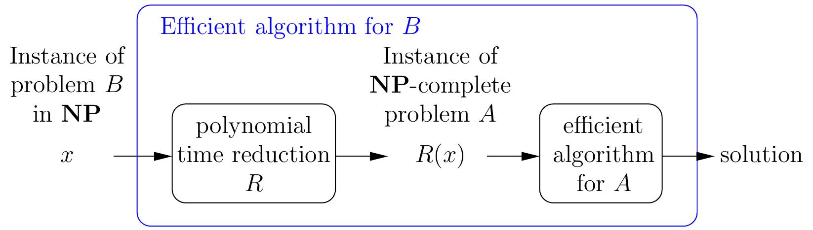
Therefore, if we have

a polynomial time reduction from $ B $ to $ A $, and
a polynomial-time algorithm solving $ A $,

then we have a polynomial-time algorithm for solving $ B $ as well: given an instance $ x $ of $ B $, compute $ R(x) $ and then run the algorithm for $ A $ on $ R(x) $.

Definition: NP-completeness

A problem $ A $ in $ \NP $ is $ \NP $-complete if every other problem $ B $ in $ \NP $ can be reduced to it with a polynomial-time computable reduction.

Therefore,

if an $ \NP $-complete problem $ A $ can be solved in polynomial time, then all the problems in $ \NP $ can, and thus
$ \NP $-complete problems are, in a sense, the most difficult ones in $ \NP $.

We do not know whether $ \NP $-complete problems can be solved efficiently or not.

The Cook-Levin Theorem¶

The fact that $ \NP $-complete problems exist at all was proven by Cook and Levin in 1970’s.

Theorem: Cook 1971, Levin 1973

$ \SAT{} $ (and $ \SATT{} $) is $ \NP $-complete.

Soon after this, Karp [1972] then listed the next 21 $ \NP $-complete problems. Since then, hundreds of problems have been shown $ \NP $-complete. For instance, $ \Prob{travelling salesperson} $, $ \Prob{generalized Sudokus} $ etc are all $ \NP $-complete. For incomplete lists, one can see

Garey and Johnson, 1979: Computers and Intractability: A Guide to the Theory of NP-Completeness, or
this wikipedia page.

How to prove a new problem NP-complete?¶

Suppose that we are given a new problem $ C $ that we suspect to be $ \NP $-complete. To prove that $ C $ is indeed $ \NP $-complete, we have to

show that it is in $ \NP $,
take any existing $ \NP $-complete problem $ A $, and
reduce $ A $ to the new problem $ C $.

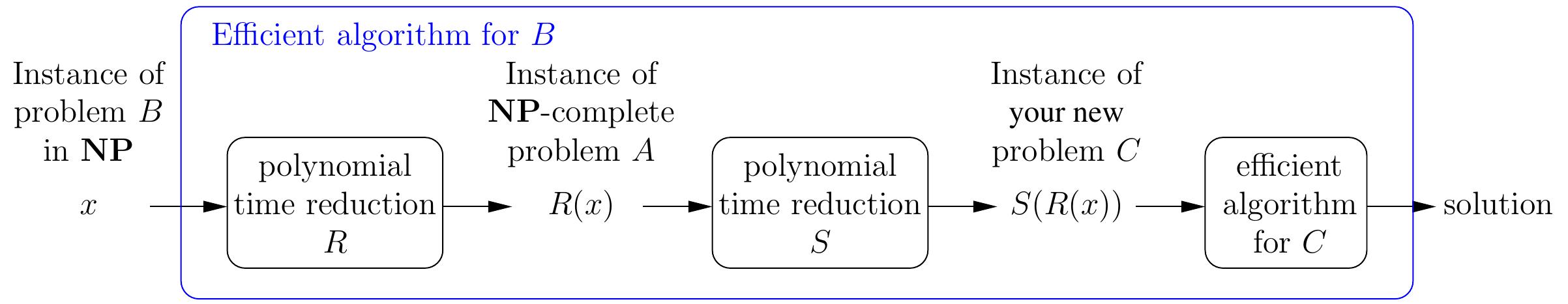
Because polynomial-time reductions compose, the existence of the reduction $ S $ from the $ \NP $-complete problem $ A $ to $ C $ actually shows that $ C $ is also $ \NP $-complete: for any problem $ B $ in $ \NP $, we can now build a reduction from $ B $ to $ C $ by

first reducing the instance $ x $ of $ B $ to an instance $ R(x) $ of $ A $ (such a reduction $ R $ exists because $ A $ is $ \NP $-complete), and
then reducing the instance $ R(x) $ to the instance $ S(R(x)) $ of $ C $. The instance $ x $ is a “yes” instance of $ B $ if and only if $ S(R(x)) $ is a “yes” instance of $ C $.

As a consequence, if the new problem $ C $ can be solved in polynomial time, then so can $ A $ and all the other problems in $ \NP $.

Usually, but not always, the first step of showing that the new problem is in $ \NP $, meaning that it has polynomial-sized certificates that can be verified in polynomial time, is easy. The real difficulty is to choose the $ \NP $-complete problem $ A $ carefully so that defining the polynomial-time reduction from $ A $ to $ C $ is as easy as possible.

Proving NP-completeness: an example¶

Consider the following problem:

Definition: $ \Prob{recruiting strangers} $

INSTANCE: A social network of students and a positive integer $ K $, where a social network consist of (i) a finite set of students and (ii) a symmetric, binary “knows” relation over the students.

QUESTION: is it possible to recruit $ K $ students so that none of these students knows each other?

Example

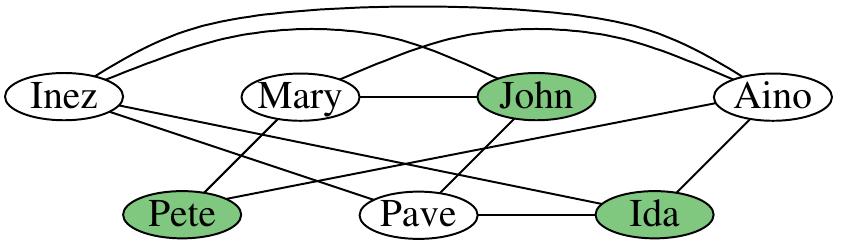
Consider the instance with the network drawn below and $ K=3 $. Is it possible to find 3 students so that none of them knows any of the others?

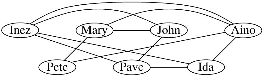
This instance is indeed a “yes” instance, the green vertices below show a solution. Is the solution the only one or are there others?

This problem is in fact equivalent to a well-known graph problem called $ \ISET $:

Definition: $ \ISET $

INSTANCE: An undirected graph $ G = (V,E) $ and an integer $ K $.

QUESTION: Is there an independent set $ I \subseteq V $, with $ \Card{I} = K $? (A set $ I \subseteq V $ is an independent set if for all distinct $ u,w \in I $, $ \Set{u,w} \notin E $.)

The $ \ISET $ problem is one of the classic $ \NP $-complete problems, let’s now show this fact with a semi-formal proof.

Theorem

$ \ISET $ is $ \NP $-complete.

Proof sketch

We reduce from the $ \SATT $ problem. We are given a 3-CNF formula $ \phi = C_1 \land … \land C_m $ with $ m $ clauses, each $ C_i = (l_{i,1} \lor l_{i,2} \lor l_{i,3}) $ having exactly three literals over distinct variables. We form the corresponding $ \ISET $ instance by letting $ K = m $ and building the graph $ G $ as follows.

For each clause $ C_i = (l_{i,1} \lor l_{i,2} \lor l_{i,3}) $, the graph contains the vertices $ v_{i,1} $, $ v_{i,2} $, and $ v_{i,3} $. Intuitively, the vertex $ v_{i,p} $ corresponds to the literal $ l_{i,p} $ (either $ x $ or $ \neg x $ for some variable $ x $) of the clause.
There is an edge between two vertices $ v_{i,p} $ and $ v_{j,q} $ if and only if either
- $ i = j $, meaning that the vertices correspond literals in the same clause, or
- $ l_{i,p} = x $ and $ l_{j,q} = \neg x $ (or vice versa) for some variable $ x $.

The first edge condition above guarantees that only one of the vertices corresponding to literals in the same clause can be selected in an independent set. The second one guarantees that if we select a vertex corresponding to a literal $ x $ in the independent set, then we cannot include any vertex corresponding to the literal $ \neg x $ (and vice versa).

Suppose that $ \phi $ is satisfied by a truth assignment $ \TA $. Then we can form the independent set $ I $ of size $ K = m $ as follows. For each clause $ C_i = (l_{i,1} \lor l_{i,2} \lor l_{i,3}) $, $ \TA(l_{i,p}) = \True $ for at least one literal in it because $ \TA $ satisfied $ \phi $: select one of such literals and include the corresponding vertex in the graph in $ I $. The set $ I $ has $ m $ elements as is an independent set because we selected only one vertex in each “clause triangle” and never selected a literal and its negation.

On the other hand, suppose that $ I $ is an independent set of size $ K = m $. In this case, we can form a truth assignment $ \TA $ that satisfies $ \phi $ as follows. For each clause $ C_i = (l_{i,1} \lor l_{i,2} \lor l_{i,3}) $, the independent set must contain exactly one of the vertices $ v_{i,1} $, $ v_{i,2} $, and $ v_{i,3} $, otherwise it could not be of size $ m $ or an independent set. Select the literal $ l $ corresponding to that vertex and let $ \TA(x) = \True $ if $ l = x $ and $ \TA(x) = \False $ if $ l = \neg x $ for a variable $ x $. After done for all the clauses, the truth assignment satisfies each of the clauses. It may still have some variables that do not have a value, let them have the value $ \False $.

As a consequence:

If $ \phi $ is satisfiable, then $ G $ has an independent set of size $ K $.
If $ G $ has an independent set of size $ K $, then $ \phi $ is satisfiable.
$ \phi $ is satisfiable if and only if $ G $ has an independent set of size $ K $.

Because of the above theorem, If we could solve $ \ISET $ in polynomial time, then we could solve $ \SAT $ and all other problems in $ \NP $ in polynomial time as well.

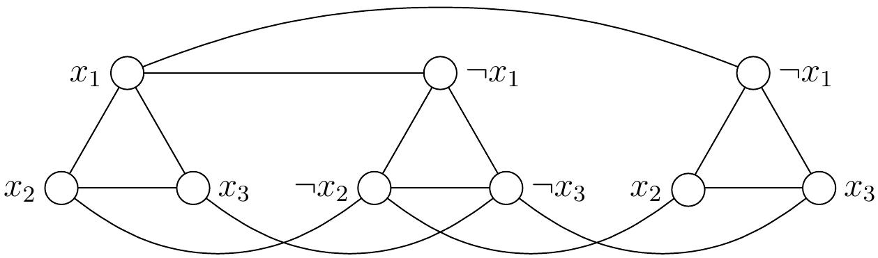
Example: Reduction from $ \SATT $ to $ \ISET $

Consider the 3-CNF formula $ \phi = (x_1 \lor x_2 \lor x_3)\land (\neg x_1 \lor \neg x_2 \lor \neg x_3) \land (\neg x_1 \lor x_2 \lor x_3) $.

The corresponding $ \ISET $ problem instance consists of the graph $ G $ below and the independent set size requirement $ K=3 $:

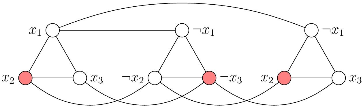
The formula $ \phi $ is satisfiable. For any satisfying truth assignment, such as $ \TA = \{x_1 \mapsto \True,x_2 \mapsto \True,x_3 \mapsto \False\} $, we can get an independent set of size 3 by taking, for each “clause triangle”, one of the vertices that correspond to a literal that evaluates to true in that clause under the assignment. For instance, the red vertices in the graph below show one possibility for the assignment $ \TA $ above.

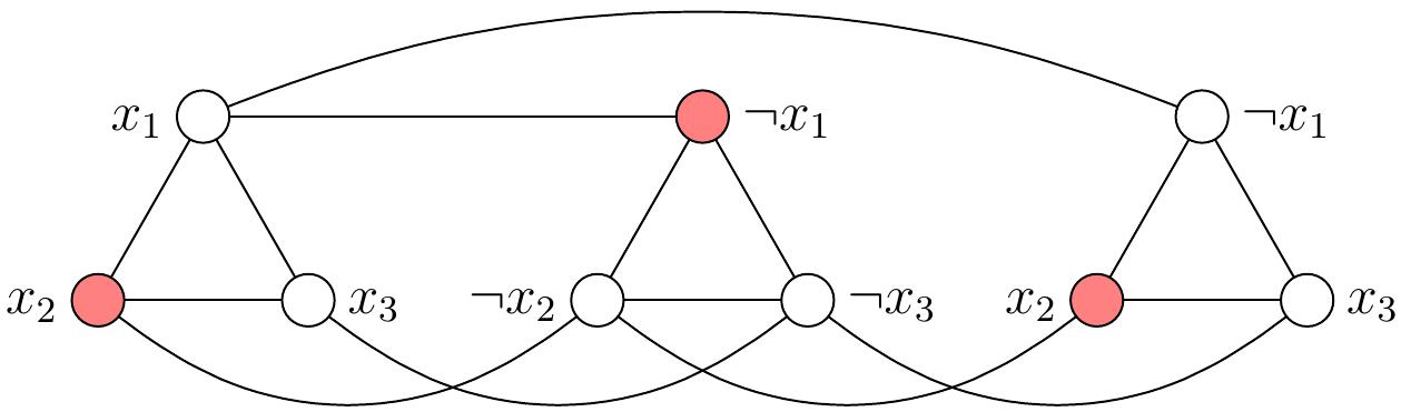
Conversely, from any independent set of size 3 in the graph, we obtain a truth assignment $ \TA $ that satisfies the formula $ \phi $ by letting $ \TA(x) = \True $ if a vertex with label $ x $ is in the independent set, and $ \TA(x) = \False $ otherwise. For instance, consider the independent set shown below in red. From this, we obtain the truth assignment $ \TA = \{x_1 \mapsto \False, x_2 \mapsto \True, x_3 \mapsto \False\} $ that satisfies $ \phi $.

Example: NP-completeness of subset-sum¶

The $ \SUBSETSUM $ problem is in $ \NP $ as we can easily check whether a set of numbers (i) is a subset of the given set of numbers, and (ii) adds to the target value $ t $. We can show that $ \SUBSETSUM $ is NP-complete by reducing $ \SATT $ to it. Suppose that we are given a CNF formula $ \phi = C_1 \land … \land C_m $, where each clause $ C_i $ contains 3 literals over distinct variables. Let the variables occurring in $ \phi $ be $ x_1,…,x_n $. We now build (in polynomial time) an instance $ \Tuple{S_{\phi},t_{\phi}} $ of $ \SUBSETSUM $ so that

$ \phi $ is satisfiable if and only if $ S_{\phi} $ has a subset summing to $ t_{\phi} $.

Therefore, if we could solve $ \SUBSETSUM $ in polynomial time, then we could solve $ \SATT $ in polynomial time as well. The polynomial-time reduction works as follows.

The numbers in $ S_{\phi} $ and $ t_{\phi} $ are base-10 numbers consisting of $ n+m $ digits $ \hat x_1 … \hat x_n \hat C_1 … \hat C_m $.
For each variable $ x_i $, the set $ S_{\phi} $ includes two numbers:
- $ v_i $ with the digit $ \hat x_i = 1 $ and the digits $ \hat C_j = 1 $ for each clause $ C_j $ containing the literal $ x_i $; the other digits are 0.
- $ v’_i $ with the digit $ \hat x_i = 1 $ and the digits $ \hat C_j = 1 $ for each clause $ C_j $ containing the literal $ \neg x_i $; the other digits are 0.
For each clause $ C_j $, the set $ S_{\phi} $ has two numbers:
- $ s_j $ with the digit $ \hat C_j = 1 $ and the other digits 0.
- $ s’_j $ with the digit $ \hat C_j = 2 $ and the other digits 0.
The target value $ t_{\phi} $ has
- the digit $ \hat x_i = 1 $ for each variable $ x_i $, and
- the digit $ \hat C_j = 4 $ for each clause $ C_j $.

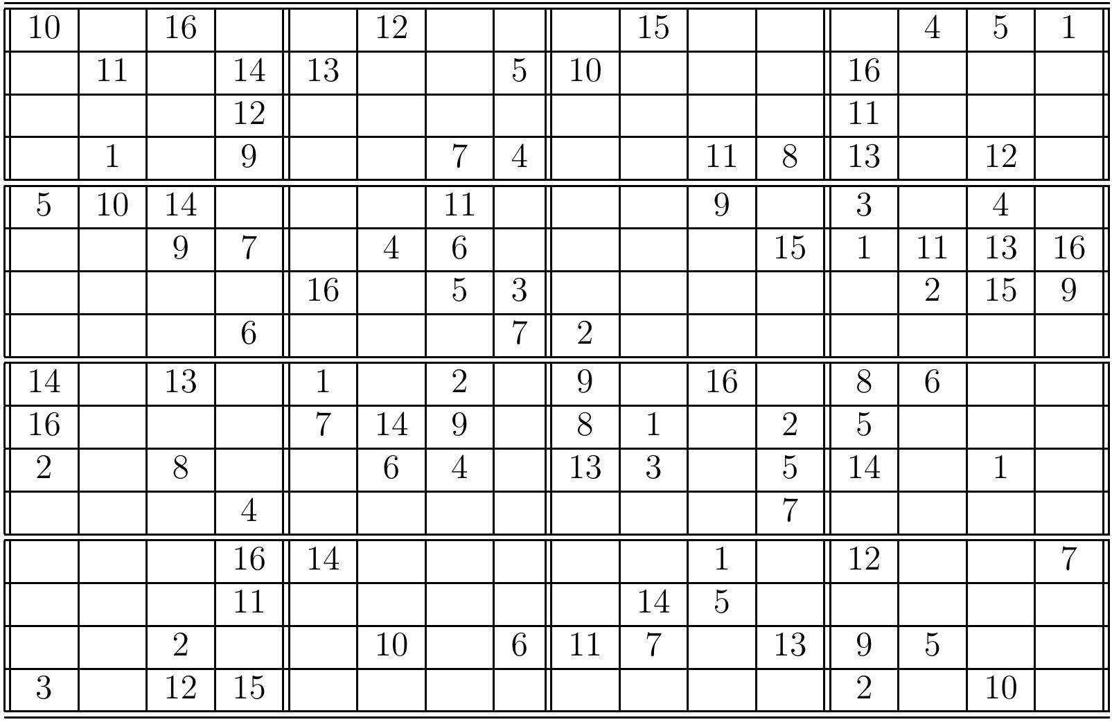
Example

Consider the 3-CNF formula $ \phi = C_1 \land C_2 \land C_3 \land C_4 $, where

$ C_1 = (x_1 \lor x_2 \lor \neg x_3) $
$ C_2 = (x_1 \lor \neg x_2 \lor x_3) $
$ C_3 = (\neg x_1 \lor x_2 \lor x_3) $
$ C_4 = (\neg x_1 \lor \neg x_2 \lor \neg x_3) $

Observe that an assignment satisfies the formula iff it assigns an even number of $ x_1 $, $ x_2 $ and $ x_3 $ to true. The corresponding $ \SUBSETSUM $ instance $ \Tuple{S_{\phi}, t_{\phi}} $, where $ S_{\phi} = \{1001100,1000011,101010,100101,10110,11001,1000,2000,100,200,10,20,1,2\} $ and $ t_{\phi} = 1114444 $, is shown below.

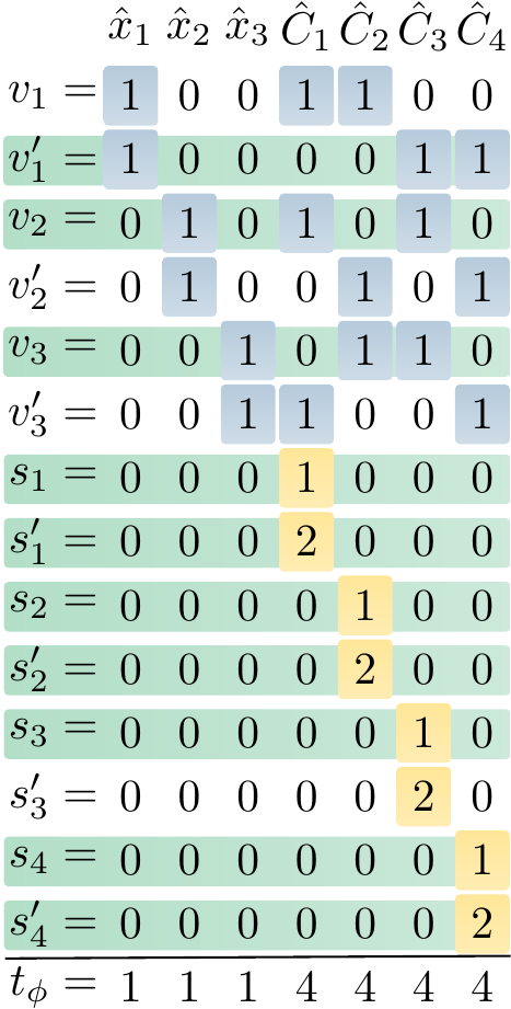
The subset $ S’ $ of $ S_{\phi} $ highlighted with green in the figure is a solution to $ \Tuple{S_{\phi}, t_{\phi}} $. The assignment $ \TA = \{x_1 \mapsto \False,x_2 \mapsto \True,x_3\mapsto\True\} $ corresponding to $ S’ $ satisfies the formula $ \phi $.

The correctness of the reduction can be argumented as follows:

Suppose that an assignment $ \TA $ satisfies $ \phi $. We can build a corresponding $ S’ \subseteq S_{\phi} $ summing to $ t_{\phi} $ as follows.
- First, for each variable $ x_i $: If $ \TA(x_i) = \True $ for a variable $ x_i $, then include $ v_i $ in $ S’ $. Otherwise, include $ v’_i $ in $ S’ $.
- At this point, the digit $ \hat C_j $ in the sum is 1, 2, or 3.
- For each clause $ C_j $, include the slack variable $ s_j $, $ s’_j $ or both so that the digit $ \hat C_j $ in the sum becomes $ 4 $.
In the other direction, suppose that a set $ S’ \subseteq S_{\phi} $ sums to $ t_{\phi} $. We build a truth assignment $ \TA $ that satisfies $ \phi $ as follows.
- First note that $ S’ $ contains either $ v_i $ or $ v’_i $ (but not both) for each variable $ x_i $ as the digit $ \hat x_i = 1 $ in $ t_{\phi} $.
- If $ v_i \in S’ $, let $ \TA(x_i) = \True $, otherwise let $ \TA(x_i) = \False $.
- Now at least one literal in each clause $ C_j $ is true under $ \TA $ because the slack variables $ s_j $ alone can only sum the digit $ \hat C_j $ up to 3 but 4 is required in $ t_{\phi} $.

NP-completeness: significance¶

Of course, the question of whether $ \Poly = \NP $, or can $ \NP $-complete problems be solved in polynomial time, is a very important open problem in computer science. In fact, it is one of the seven (of which six are still open) one million dollar prize Clay Mathematics Institute Millennium Prize problems.

Because there are hundreds of $ \NP $-complete problems, the $ \Poly = \NP $ question has practical significance as well. As Christos Papadimitriou says in his book “Computational complexity”:

There is nothing wrong in trying to prove that an $ \NP $-complete problem can be solved in polynomial time. The point is that without an $ \NP $-completeness proof one would be trying the same thing without knowing it!

That is, suppose that you have a new problem for which you should develop an algorithm that is always efficient, i.e. runs in polynomial time. You may end up in trying really hard for very long time, probably without success, if the problem turns out to be $ \NP $-complete or harder. This is because during the last decades, lots of very clever people have tried to develop polynomial-time algorithms for many $ \NP $-complete problems, but no-one has succeeded so far.

So what to do when a problem is $ \NP $-complete? As there are lots practical problems that have to be solved even though they are $ \NP $-complete (or even harder), one has to develop some approaches that work “well enough” in practise. Some alternatives are:

Develop backtracking search algorithms with efficient heuristics and pruning techniques.
Attack some special cases occurring in practise.
Develop approximation algorithms.
Apply incomplete local search methods.
Use existing tools.

Exhaustive search¶

Perhaps the simplest way to solve computationally harder problems is to exhaustively search through all the solution candidates. This is usually done with a backtracking search that tries to build a solution by extending partial solutions to larger ones. Of course, in the worst case this takes superpolynomial, usually exponential or worse, time for $ \NP $-complete and more difficult problems However, for some instances the search may quickly find a solution or deduce that there is none. The search can usually be improved by adding clever pruning techniques that help detecting earlier that a partial solution cannot be extended to a full solution.

As an example, recall the following simple recursive backtracking search algorithm for the $ \SUBSETSUM $ problem introduced in the CS-A1120 Programming 2 course:

def solve(set: Set[Int], target: Int): Option[Set[Int]] = {
  def inner(s: Set[Int], t: Int): Option[Set[Int]] = {
    if(t == 0) return Some(Set[Int]())
    else if (s.isEmpty) return None
    val e = s.head
    val rest = s - e
    // Search for a solution without e
    val solNotIn = inner(rest, t)
    if (solNotIn.nonEmpty) return solNotIn
    // Search for a solution with e
    val solIn = inner(rest, t - e)
    if (solIn.nonEmpty) return Some(solIn.get + e)
    // No solution found here, backtrack
    return None
  }
  inner(set, target)
}

For the instance in which $ S = \Set{-9,-3,7,12} $ and $ t = 10 $, the call tree of the above program looks like this:

The search procedure can be improved by adding a pruning rule that detects whether the target value is too large or too small so that the number in the set $ S $ can never sum to it:

def solve(set: Set[Int], target: Int): Option[Set[Int]] = {
  def inner(s: Set[Int], t: Int): Option[Set[Int]] = {
    if(t == 0) return Some(Set[Int]())
    else if (s.isEmpty) return None
    else if (s.filter(_ > 0).sum < t || s.filter(_ < 0).sum > t)
      // The positive (negative) number cannot add up (down) to t
      return None
    val e = s.head
    val rest = s - e
    // Search for a solution without e
    val solNotIn = inner(rest, t)
    if (solNotIn.nonEmpty) return solNotIn
    // Search for a solution with e
    val solIn = inner(rest, t - e)
    if (solIn.nonEmpty) return Some(solIn.get + e)
    // No solution found here, backtrack
    return None
  }
  inner(set, target)
}

Now the call tree for the same instance as above, $ S= \Set{-9,-3,7,12} $ and $ t = 10 $, is smaller because some of the search branches get terminated earlier:

Special cases¶

Sometimes we have a computationally hard problem but the instances that occur in practise are somehow restricted special cases. In such a case, it may be possible to develop an algorithm that solves such special instances efficiently. Technically, we are not solving the original problem anymore but a different problem where the instance set is a subset of the original problem instance set.

Example: subset-sum with smallish values¶

In the case of $ \SUBSETSUM $, it is quite easy to develop a dynamic programming (recall Round 6) algorithm that works extremely well for “smallish” numbers. First, define a recursive function $ \SSDP(S,t) $ evaluating to true if and only if $ S = \Set{v_1,v_2,…,v_n} $ has a subset that sums to $ t $:

$ \SSDP(S,t) = \True $ if $ t = 0 $,
$ \SSDP(S,t) = \False $ if $ S = \emptyset $ and $ t \neq 0 $,
$ \SSDP(S,t) = \True $ if $ \SSDP(\Set{v_2,v_3,…,v_n},t)=\True $ or $ \SSDP(\Set{v_2,v_3,…,v_n},t-v_1)=\True $, and
$ \SSDP(S,t) = \False $ otherwise.

Now, using the memoization technique with arrays, it is easy to implement a dynamic programming algorithm that works in time $ \Oh{\Card{S} M} $ and needs $ \Oh{M \log_2 M} $ bytes of memory, where $ M = \sum_{s \in S,s > 0}s - \sum_{s \in S,s < 0}s $ is the size of the range in which the sums of all possible subsets of $ S $ must be included. Solution reconstruction is also rather straightforward. Algorithm sketch:

Take an empty array $ a $.
For each number $ x \in S $ in turn, insert in one pass
- $ a[y+x] = x $ for each $ y $ for which $ a[y] $ is already defined, and
- $ a[x] = x $.

That is, in a number-by-number manner, insert all the subset sums that can be obtained either using the number alone or by adding it to any of the sums obtainable by using earlier numbers. The value written in the element $ a[s] $ tells what was the last number inserted to get the sum $ s $; this allows reconstruction of the solution subset.

Example

Assume that the set of numbers is $ S= \Set{2,7,14,49,98,343,686,2409,2793,16808,17206,117705,117993} $. The beginning of the array is

Inspecting the array, one can directly see that, for instance, there is a subset $ S’ \subseteq S $ for which $ \sum_{s \in S’} = 58 $ and that such a subset is obtained with the numbers $ a[58] = 49 $, $ a[58-49] = a[9] = 7 $ and $ a[9-7] = a[2] = 2 $.

Is the dynamic programming algorithm above a polynomial time algorithm for the $ \NP $-complete problem $ \SUBSETSUM $? No, unfortunately it is not:

the size of the input instance is the number of bits needed to represent the numbers, and
therefore the value of the sum $ \sum_{s \in S,s > 0}s - \sum_{s \in S,s < 0}s $, and thus the running time as well, can be exponentially large with respect to the instance size.

For instance, the numbers that were produced in our earlier reduction from $ \SATT $ to $ \SUBSETSUM $ are not small: if the $ \SATT $ instance has $ n $ variables and $ m $ clauses, then the numbers have $ n+m $ digits and their values are in the order $ 10^{n+m} $, i.e., exponential in $ n+m $. Note: if the dynamic programming approach is implemented with hash maps instead of arrays, then it works for the special case when the numbers are not necessarily “smallish” but when the number of different sums that can be formed from $ S $ is “smallish”.

Reducing to an another problem¶

For some $ \NP $-complete and harder problems there are some very sophisticated solver tools that work extremely well for many practical instances:

propositional satisfiability: MiniSat and others
integer linear programming (ILP): lp_solve and others
satisfiability modulo theories: Z3 and others
and many others …

Thus if one can reduce the current problem $ B $ into one of the problems $ A $ above, it may be possible to obtain a practically efficient solving method without programming the search method by one-self. Notice that here we are using reductions in the other direction compared to the case when we proved problems $ \NP $-complete: we now take the problem which we would like to solve and reduce it a problem for which we have an usually-efficient tool available:

Example: solving Sudokus with SAT¶

Let us apply the above described approach to Sudoku solving. Our goal is to use the sophisticated CNF SAT solvers available. Thus, given an $ n \times n $ partially filled Sudoku grid, we want to make a propositional formula $ \phi $ such that

the Sudoku grid has a solution if and only the formula is satisfiable, and
from a satisfying assignment for $ \phi $ we can build a solution for the Sudoku grid.

In practise we thus want to use the following procedure:

To obtain such a CNF formula $ \phi $ for a Sudoku grid, we first introduce a variable $$\SUD{r}{c}{v}$$ for each row $ r = 1,…,n $, column $ c = 1,…,n $ and value $ v = 1,…,n $. The intuition is that if $ \SUD{r}{c}{v} $ is true, then the grid element at row $ r $ and column $ c $ has the value $ v $. The formula $$\phi = C_1 \land C_2 \land C_3 \land C_4 \land C_5 \land C_6$$ is built by introducing sets of clauses that enforce different aspects of the solution:

Each entry has at least one value: $ C_1 = \bigwedge_{1 \le r \le n, 1 \le c \le n}(\SUD{r}{c}{1} \lor \SUD{r}{c}{2} \lor … \lor \SUD{r}{c}{n}) $
Each entry has at most one value: $ C_2 = \bigwedge_{1 \le r \le n, 1 \le c \le n,1 \le v < v’ \le n}(\neg\SUD{r}{c}{v} \lor \neg\SUD{r}{c}{v’}) $
Each row has all the numbers: $ C_3 = \bigwedge_{1 \le r \le n, 1 \le v \le n}(\SUD{r}{1}{v} \lor \SUD{r}{2}{v} \lor … \lor \SUD{r}{n}{v}) $
Each column has all the numbers: $ C_4 = \bigwedge_{1 \le c \le n, 1 \le v \le n}(\SUD{1}{c}{v} \lor \SUD{2}{c}{v} \lor … \lor \SUD{n}{c}{v}) $
Each block has all the numbers: $ C_5 = \bigwedge_{1 \le r’ \le \sqrt{n}, 1 \le c’ \le \sqrt{n}, 1 \le v \le n}(\bigvee_{(r,c) \in B_n(r’,c’)}\SUD{r}{c}{v}) $ where $ B_n(r’,c’) = \Setdef{(r’\sqrt{n}+i,c’\sqrt{n}+j)}{0 \le i < \sqrt{n}, 0 \le j < \sqrt{n}} $
The solution respects the given cell values $ \SUDHints $: $ C_6 = \bigwedge_{(r,c,v) \in \SUDHints}(\SUD{r}{c}{v}) $

The resulting formula has $ \Card{\SUDHints} $ unary clauses, $ n^2\frac{n(n-1)}{2} $ binary clauses, and $ 3n^2 $ clauses of length $ n $. Thus the size of the formula is polynomial with respect to $ n $.

Example

Consider the following Sudoku grid:

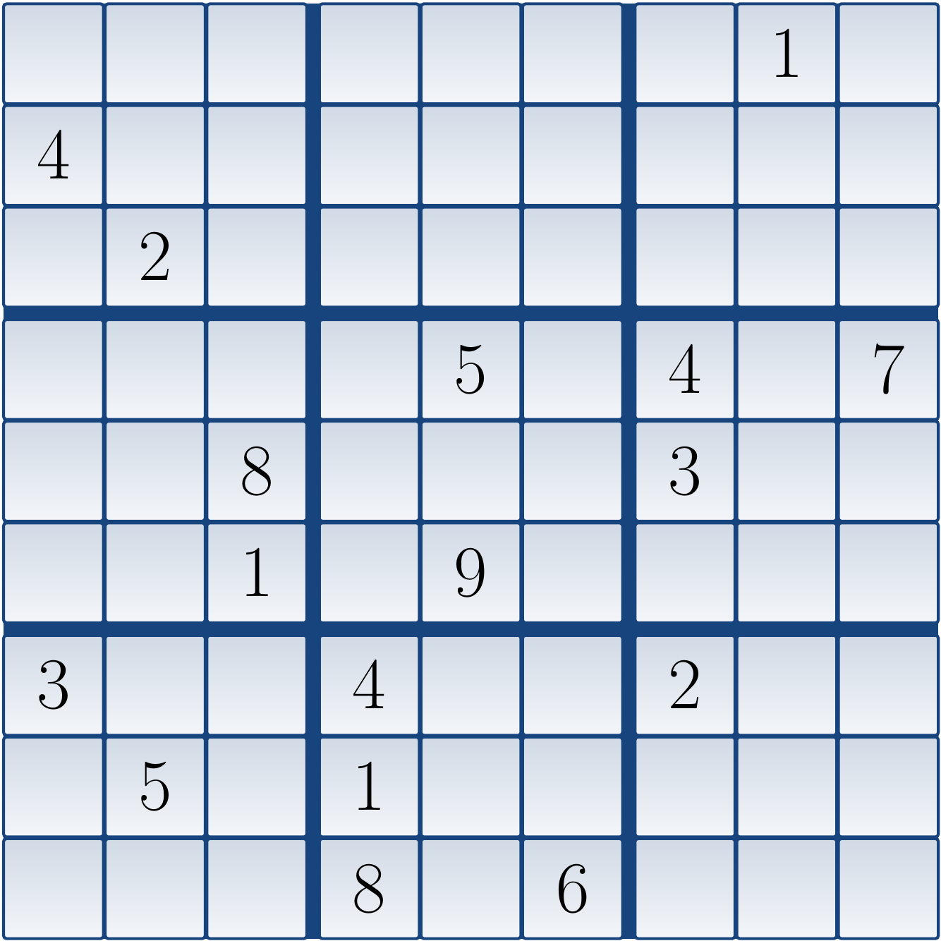
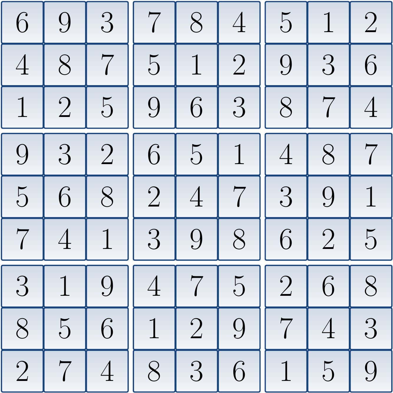
The corresponding CNF formula is: \begin{eqnarray*} (x_{1,1,1} \lor x_{1,1,2} \lor … \lor x_{1,1,9}) \land … \land (x_{9,9,1} \lor x_{9,9,2} \lor … \lor x_{9,9,9}) &\land&\\ (\neg x_{1,1,1} \lor \neg x_{1,1,2}) \land … \land (\neg x_{9,9,8} \lor \neg x_{9,9,9}) &\land&\\ (x_{1,1,1} \lor x_{1,2,1} \lor … \lor x_{1,9,1}) \land … \land (x_{9,1,9} \lor x_{9,2,9} \lor … \lor x_{9,9,9}) &\land&\\ (x_{1,1,1} \lor x_{2,1,1} \lor … \lor x_{9,1,1}) \land … \land (x_{1,9,9} \lor x_{2,9,9} \lor … \lor x_{9,9,9}) &\land&\\ (x_{1,1,1} \lor x_{1,2,1} \lor … \lor x_{3,3,1}) \land … \land (x_{7,7,9} \lor x_{7,8,9} \lor … \lor x_{9,9,9}) &\land&\\ (x_{1,8,1}) \land (x_{2,1,4}) \land (x_{3,2,2}) \land … \land (x_{9,6,6})&& \end{eqnarray*} When the formula is given to a SAT solver, it declares that the formula has a model in which all $ x_{1,1,i} $ except $ x_{1,1,6} $ are false, and so on. From the variables that are true, we obtain the following (unique) solution to the original Sudoku grid:

An implementation of this approach, using the Sat4j SAT solver implemented in Java, is available in the Eclipse package for the “coloring with SAT” programming exercise. Feel free to compare its performance to the Sudoku solver you implemented in the CS-A1120 Programming 2 course.

Note

This approach of describing an instance of some other problem as a satisfiability instance, or an instance of some other similar constraint satisfaction formalism, is also called constraint programming.

It is a form of declarative programming: one only declares how the solution should look like and then a constraint solver finds one (or states that none exists).

Further references¶

Sanjeev Arora and Boaz Barak, Computational Complexity: A Modern Approach